This post isn’t about upcoming features, it’s about things you can already do with Profiler. What we’ll see is how to import structures used for file system analysis from C/C++ sources, use them to analyze raw hex data, create a script to do the layout work for us in the future and at the end we’ll see how to create a little utility to recover deleted files. The file system used for this demonstration is FAT32, which is simple enough to avoid making the post too long.
Note: Before starting you might want to update. The 1.0.1 version is out and contains few small fixes. Among them the ‘signed char’ type wasn’t recognized by the CFFStruct internal engine and the FAT32 structures I imported do use it. While ‘signed char’ may seem redundant, it does make sense, since C compilers can be instructed to treat char types as unsigned.
Import file system structures
Importing file system structures from C/C++ sources is easy thanks to the Header Manager tool. In fact, it took me less than 30 minutes to import the structures for the most common file systems from different code bases. Click here to download the archive with all the headers.
Here’s the list of headers I have created:
- ext – ext2/3/4 imported from FreeBSD
- ext2 – imported from Linux
- ext3 – imported from Linux
- ext4 – imported from Linux
- fat – imported from FreeBSD
- hfs – imported from Darwin
- iso9660 – imported from FreeBSD
- ntfs – imported from Linux
- reiserfs – imported from Linux
- squashfs – imported from Linux
- udf – imported from FreeBSD
Copy the files to your user headers directory (e.g. “AppData\Roaming\CProfiler\headers”). It’s better to not put them in a sub-directory. Please note that apart from the FAT structures, none of the others have been tried out.
Note: Headers created from Linux sources contain many additional structures, this is due to the includes in the parsed source code. This is a bit ugly: in the future it would be a good idea to add an option to import only structures belonging to files in a certain path hierarchy and those referenced by them.
Since this post is about FAT, we’ll see how to import the structures for this particular file system. But the same steps apply for other file systems as well and not only for them. If you’ve never imported structures before, you might want to take a look at this previous post about dissecting an ELF and read the documentation about C++ types.
We open the Header Manager and configure some basic options like ‘OS’, ‘Language’ and ‘Standard’. In this particular case I imported the structures from FreeBSD, so I just set ‘freebsd’, ‘c’ and ‘c11’. Then we need to add the header paths, which in my case were the following:
C:/Temp/freebsd-master
C:/Temp/freebsd-master/include
C:/Temp/freebsd-master/sys
C:/Temp/freebsd-master/sys/x86
C:/Temp/freebsd-master/sys/i386/include
C:/Temp/freebsd-master/sys/i386
Then in the import edit we insert the following code:
HEADER_START("fat");

#include
#include
#include
#include
#include
Now we can click on ‘Import’.
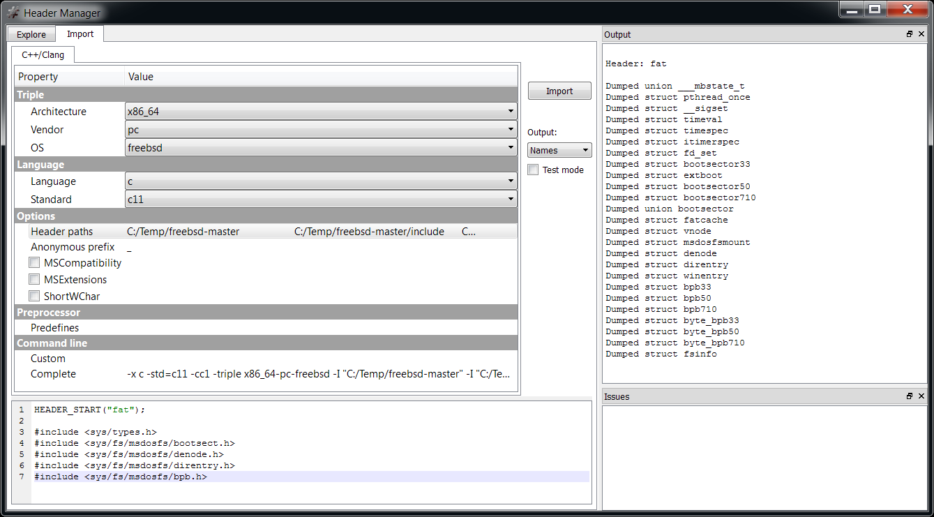
That’s it! We now have all the FAT structures we need in the ‘fat’ header file.
It should also be mentioned that I modified some fields of the direntry structure from the Header Manager, because they were declared as byte arrays, but should actually be shown as short and int values.
Parse the Master Boot Record
Before going on with the FAT analysis, we need to briefly talk about the MBR. FAT partitions are usually found in a larger container, like a partitioned device.
To perform my tests I created a virtual hard-disk in Windows 7 and formatted it with FAT32.
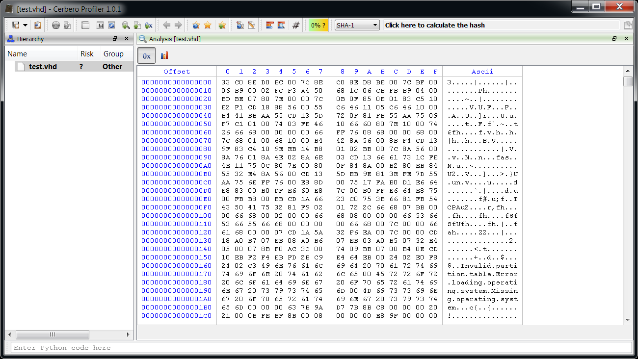
As you might be able to spot, the VHD file begins with a MBR. In order to locate the partitions it is necessary to parse the MBR first. The format of the MBR is very simple and you can look it up on Wikipedia. In this case we’re only interested in the start and size of each partition.
Profiler doesn’t yet support the MBR format, although it might be added in the future. In any case, it’s easy to add the missing feature: I wrote a small hook which parses the MBR and adds the partitions as embedded objects.
Here’s the cfg data:
[GenericMBR]
label = Generic MBR Partitions
file = generic_mbr.py
scanning = scanning
And here’s the Python script:
def scanning(sp, ud):
    # make sure we're at the first level and that the format is unknown
    if sp.scanNesting() != 0 or sp.getObjectFormat() != "":
        return
    # check boot signature
    obj = sp.getObject()
    bsign = obj.Read(0x1FE, 2)
    if len(bsign) != 2 or bsign[0] != 0x55 or bsign[1] != 0xAA:
        return
    # add partitions
    for x in range(4):
        entryoffs = 0x1BE + (x * 0x10)
        offs, ret = obj.ReadUInt32(entryoffs + 8)
        size, ret = obj.ReadUInt32(entryoffs + 12)
        if offs != 0 and size != 0:
            sp.addEmbeddedObject(offs * 512, size * 512, "?", "Partition #" + str(x + 1))
And now we can inspect the partitions directly (do not forget to enable the hook from the extensions).
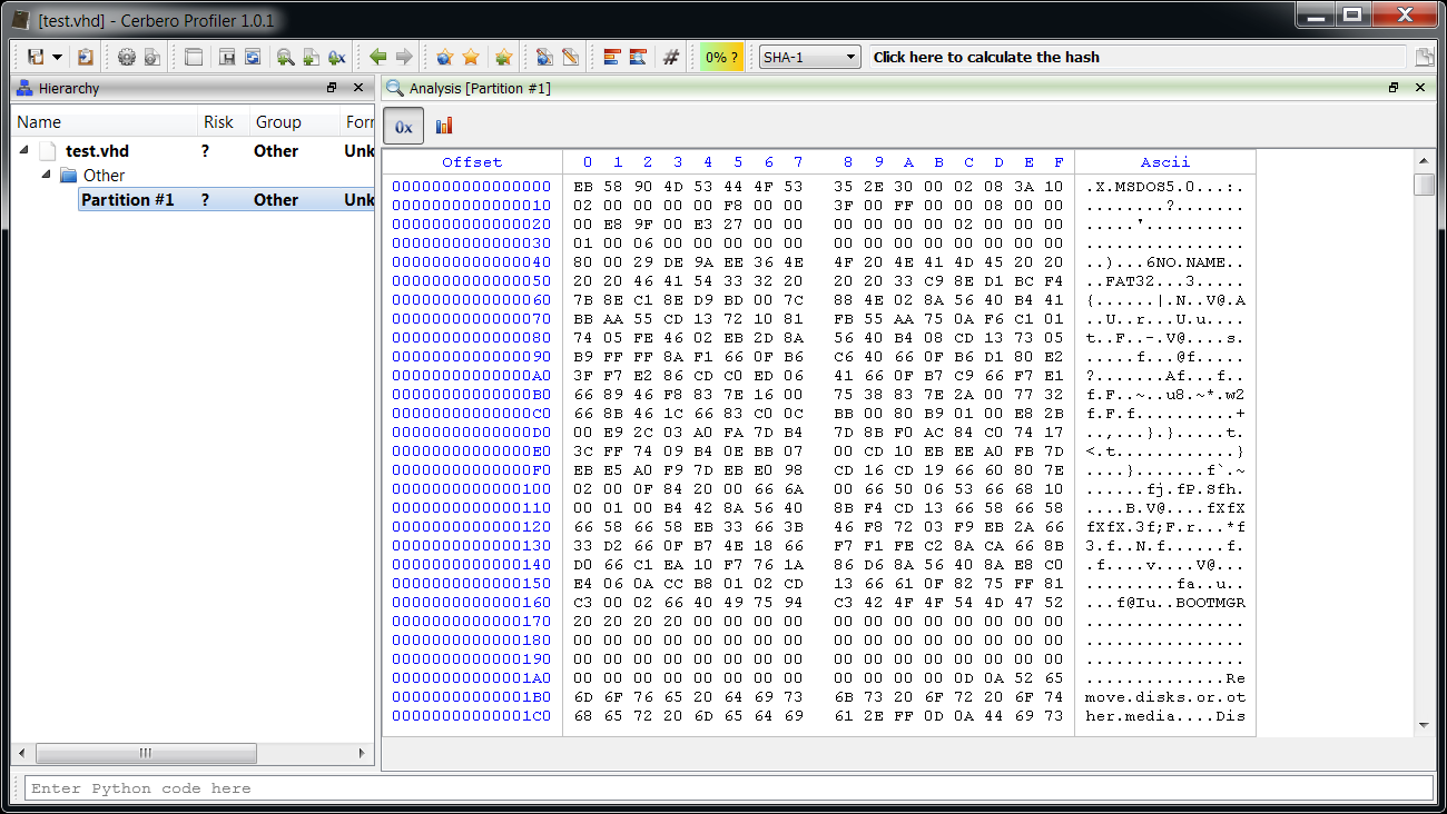
Easy.
Analyze raw file system data
The basics of the FAT format are quite simple to describe. The data begins with the boot sector header and some additional fields for FAT32 over FAT16 and for FAT16 over FAT12. We’re only interested in FAT32, so to simplify the description I will only describe this particular variant. The boot sector header specifies essential information such as sector size, sectors in clusters, number of FATs, size of FAT etc. It also specifies the number of reserved sectors. These reserved sectors start with the boot sector and where they end the FAT begins.
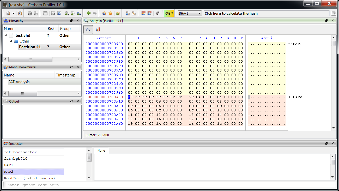
The ‘FAT’ in this case is not just the name of the file system, but the File Allocation Table itself. The size of the FAT, as already mentioned, is specified in the boot sector header. Usually, for data-loss prevention, more than one FAT is present. Normally there are two FATs: the number is specified in the boot sector header. The backup FAT follows the first one and has the same size. The data after the FAT(s) and right until the end of the partition includes directory entries and file data. The cluster right after the FAT(s) usually starts with the Root Directory entry, but even this is specified in the boot sector header.
The FAT itself is just an array of 32-bit indexes pointing to clusters. The first 2 indexes are special: they specify the range of EOF values for indexes. It works like this: a directory entry for a file (directories and files share the same structure) specifies the first cluster of said file, if the file is bigger than one cluster, the FAT is looked up at the index representing the current cluster, this index specifies the next cluster belonging to the file. If the index contains one of the values in the EOF range, the file has no more clusters or perhaps contains a damaged cluster (0xFFFFFFF7). Indexes with a value of zero are marked as free. Cluster index are 2-based: cluster 2 is actually cluster 0 in the data region. This means that if the Root Directory is specified to be located at cluster 2, it is located right after the FATs.
Hence, the size of the FAT depends on the size of the partition, and it must be big enough to accommodate an array large enough to represent every cluster in the data area.
So, let’s perform our raw analysis by adding the boot sector header and the additional FAT32 fields:
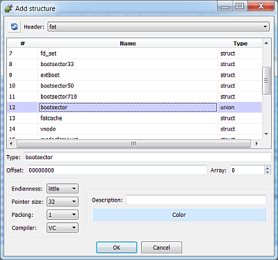
Note: When adding a structure make sure that it’s packed to 1, otherwise field alignment will be wrong.
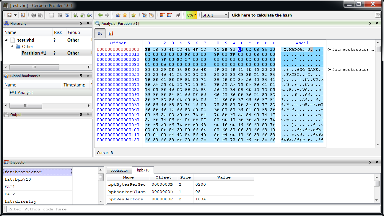
Then we highlight the FATs.
And the Root Directory entry.
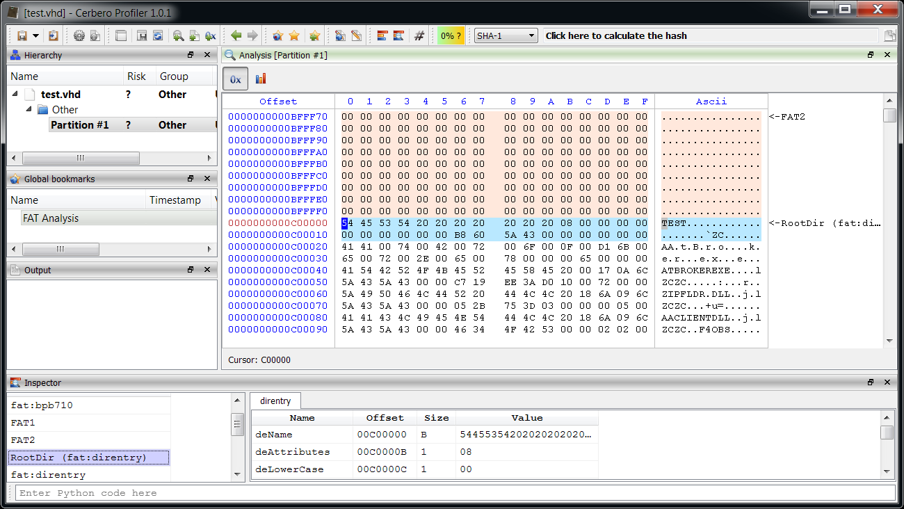
This last step was just for demonstration, as we’re currently not interested in the Root Directory. Anyway, now we have a basic layout of the FAT to inspect and this is useful.
Let’s now make our analysis applicable to future cases.
Automatically create an analysis layout
Manually analyzing a file is very useful and it’s the first step everyone of us has to do when studying an unfamiliar file format. However, chances are that we have to analyze files with the same format in the future.
That’s why we could write a small Python script to create the analysis layout for us. We’ve already seen how to do this in the post about dissecting an ELF.
Here’s the code:
from Pro.Core import *
from Pro.UI import *

def buildFATLayout(obj, l):
    hname = "fat"
    hdr = CFFHeader()
    if hdr.LoadFromFile(hname) == False:
        return
    sopts = CFFSO_VC | CFFSO_Pack1
    d = LayoutData()
    d.setTypeOptions(sopts)

    # add boot sector header and FAT32 fields
    bhdr = obj.MakeStruct(hdr, "bootsector", 0, sopts)
    d.setColor(ntRgba(0, 170, 255, 70))
    d.setStruct(hname, "bootsector")
    l.add(0, bhdr.Size(), d)
    bexhdr = obj.MakeStruct(hdr, "bpb710", 0xB, sopts)
    d.setStruct(hname, "bpb710")
    l.add(0xB, bexhdr.Size(), d)

    # get FAT32 info
    bytes_per_sec = bexhdr.Num("bpbBytesPerSec")
    sec_per_clust = bexhdr.Num("bpbSecPerClust")
    res_sect = bexhdr.Num("bpbResSectors")
    nfats = bexhdr.Num("bpbFATs")
    fat_sects = bexhdr.Num("bpbBigFATsecs")
    root_clust = bexhdr.Num("bpbRootClust")
    bytes_per_clust = bytes_per_sec * sec_per_clust

    # add FAT intervals, highlight copies with a different color
    d2 = LayoutData()
    d2.setColor(ntRgba(255, 255, 127, 70))
    fat_start = res_sect * bytes_per_sec
    fat_size = fat_sects * bytes_per_sec
    d2.setDescription("FAT1")
    l.add(fat_start, fat_size, d2)
    # add copies
    d2.setColor(ntRgba(255, 170, 127, 70))
    for x in range(nfats - 1):
        fat_start = fat_start + fat_size
        d2.setDescription("FAT" + str(x + 2))
        l.add(fat_start, fat_size, d2)
    fat_end = fat_start + fat_size

    # add root directory
    rootdir_offs = (root_clust - 2) + fat_end
    rootdir = obj.MakeStruct(hdr, "direntry", rootdir_offs, sopts)
    d.setStruct(hname, "direntry")
    d.setDescription("Root Directory")
    l.add(rootdir_offs, rootdir.Size(), d)


hv = proContext().getCurrentView()
if hv.isValid() and hv.type() == ProView.Type_Hex:
    c = hv.getData()
    obj = CFFObject()
    obj.Load(c)
    lname = "FAT_ANALYSIS" # we could make the name unique
    l = proContext().getLayout(lname)
    buildFATLayout(obj, l)
    # apply the layout to the current hex view
    hv.setLayoutName(lname)
We can create an action with this code or just run it on the fly with Ctrl+Alt+R.
Recover deleted files
Now that we know where the FAT is located and where the data region begins, we can try to recover deleted files. There’s more than one possible approach to this task (more on that later). What I chose to do is to scan the entire data region for file directory entries and to perform integrity checks on them, in order to establish that they really are what they seem to be.
Let’s take a look at the original direntry structure:
struct direntry {
	u_int8_t	deName[11];	/* filename, blank filled */
#define	SLOT_EMPTY	0x00		/* slot has never been used */
#define	SLOT_E5		0x05		/* the real value is 0xe5 */
#define	SLOT_DELETED	0xe5		/* file in this slot deleted */
	u_int8_t	deAttributes;	/* file attributes */
#define	ATTR_NORMAL	0x00		/* normal file */
#define	ATTR_READONLY	0x01		/* file is readonly */
#define	ATTR_HIDDEN	0x02		/* file is hidden */
#define	ATTR_SYSTEM	0x04		/* file is a system file */
#define	ATTR_VOLUME	0x08		/* entry is a volume label */
#define	ATTR_DIRECTORY	0x10		/* entry is a directory name */
#define	ATTR_ARCHIVE	0x20		/* file is new or modified */
	u_int8_t	deLowerCase;	/* NT VFAT lower case flags */
#define	LCASE_BASE	0x08		/* filename base in lower case */
#define	LCASE_EXT	0x10		/* filename extension in lower case */
	u_int8_t	deCHundredth;	/* hundredth of seconds in CTime */
	u_int8_t	deCTime[2];	/* create time */
	u_int8_t	deCDate[2];	/* create date */
	u_int8_t	deADate[2];	/* access date */
	u_int8_t	deHighClust[2];	/* high bytes of cluster number */
	u_int8_t	deMTime[2];	/* last update time */
	u_int8_t	deMDate[2];	/* last update date */
	u_int8_t	deStartCluster[2]; /* starting cluster of file */
	u_int8_t	deFileSize[4];	/* size of file in bytes */
};
Every directory entry has to be aligned to 0x20. If the file has been deleted the first byte of the deName field will be set to SLOT_DELETED (0xE5). That’s the first thing to check. The directory name should also not contain certain values like 0x00. According to Wikipedia, the following values aren’t allowed:
- ” * / : < > ? \ |
Windows/MS-DOS has no shell escape character - + , . ; = [ ]
They are allowed in long file names only. - Lower case letters a–z
Stored as A–Z. Allowed in long file names. - Control characters 0–31
- Value 127 (DEL)
We can use these rules to validate the short file name. Moreover, certain directory entries are used only to store long file names:
/*
 * Structure of a Win95 long name directory entry
 */
struct winentry {
	u_int8_t	weCnt;
#define	WIN_LAST	0x40
#define	WIN_CNT		0x3f
	u_int8_t	wePart1[10];
	u_int8_t	weAttributes;
#define	ATTR_WIN95	0x0f
	u_int8_t	weReserved1;
	u_int8_t	weChksum;
	u_int8_t	wePart2[12];
	u_int16_t	weReserved2;
	u_int8_t	wePart3[4];
};
We can exclude these entries by making sure that the deAttributes/weAttributes isn’t ATTR_WIN95 (0xF).
Once we have confirmed the integrity of the file name and made sure it’s not a long file name entry, we can validate the deAttributes. It should definitely not contain the flags ATTR_DIRECTORY (0x10) and ATTR_VOLUME (8).
Finally we can make sure that deFileSize isn’t 0 and that deHighClust combined with deStartCluster contains a valid cluster index.
It’s easier to write the code than to talk about it. Here’s a small snippet which looks for deleted files and prints them to the output view:
from Pro.Core import *

class FATData(object):
    pass

def setupFATData(obj):
    hdr = CFFHeader()
    if hdr.LoadFromFile("fat") == False:
        return None
    bexhdr = obj.MakeStruct(hdr, "bpb710", 0xB, CFFSO_VC | CFFSO_Pack1)
    fi = FATData()
    fi.obj = obj
    fi.hdr = hdr
    # get FAT32 info
    fi.bytes_per_sec = bexhdr.Num("bpbBytesPerSec")
    fi.sec_per_clust = bexhdr.Num("bpbSecPerClust")
    fi.res_sect = bexhdr.Num("bpbResSectors")
    fi.nfats = bexhdr.Num("bpbFATs")
    fi.fat_sects = bexhdr.Num("bpbBigFATsecs")
    fi.root_clust = bexhdr.Num("bpbRootClust")
    fi.bytes_per_clust = fi.bytes_per_sec * fi.sec_per_clust
    fi.fat_offs = fi.res_sect * fi.bytes_per_sec
    fi.fat_size = fi.fat_sects * fi.bytes_per_sec
    fi.data_offs = fi.fat_offs + (fi.fat_size * fi.nfats)
    fi.data_size = obj.GetSize() - fi.data_offs
    fi.data_clusters = fi.data_size // fi.bytes_per_clust
    return fi

invalid_short_name_chars = [
    127,
    ord('"'), ord("*"), ord("/"), ord(":"), ord("<"), ord(">"), ord("?"), ord("\\"), ord("|"),
    ord("+"), ord(","), ord("."), ord(";"), ord("="), ord("["), ord("]")
    ]
def validateShortName(name):
    n = len(name)
    for x in range(n):
        c = name[x]
        if (c >= 0 and c <= 31) or (c >= 0x61 and c <= 0x7A) or c in invalid_short_name_chars:
            return False
    return True

# validate short name
# validate attributes: avoid long file name entries, directories and volumes
# validate file size
# validate cluster index
def validateFileDirectoryEntry(fi, de):
    return validateShortName(de.name) and de.attr != 0xF and (de.attr & 0x18) == 0 and \
            de.file_size != 0 and de.clust_idx >= 2 and de.clust_idx - 2 < fi.data_clusters

class DirEntryData(object):
    pass

def getDirEntryData(b):
    # reads after the first byte
    de = DirEntryData()
    de.name = b.read(10)
    de.attr = b.u8()
    b.read(8) # skip some fields
    de.high_clust = b.u16()
    b.u32() # skip two fields
    de.clust_idx = (de.high_clust << 16) | b.u16()
    de.file_size = b.u32()
    return de

def findDeletedFiles(fi):
    # scan the data region one cluster at a time using a buffer
    # this is more efficient than using an array of CFFStructs
    dir_entries = fi.data_size // 0x20
    b = fi.obj.ToBuffer(fi.data_offs)
    b.setBufferSize(0xF000)
    for x in range(dir_entries):
        try:
            unaligned = b.getOffset() % 0x20
            if unaligned != 0:
                b.read(0x20 - unaligned)
            # has it been deleted?
            if b.u8() != 0xE5:
                continue
            # validate fields
            de = getDirEntryData(b)
            if validateFileDirectoryEntry(fi, de) == False:
                continue
            # we have found a deleted file entry!
            name = de.name.decode("ascii", "replace")
            print(name + " - offset: " + hex(b.getOffset() - 0x20))
        except:
            # an exception occurred, debug info
            print("exception at offset: " + hex(b.getOffset() - 0x20))
            raise

obj = proCoreContext().currentScanProvider().getObject()
fi = setupFATData(obj)
if fi != None:
    findDeletedFiles(fi)
This script is to be run on the fly with Ctrl+Alt+R. It's not complete, otherwise I would have added a wait box, since like it's now the script just blocks the UI for the entire execution. We'll see later how to put everything together in a meaningful way.
The output of the script is the following:
���������� - offset: 0xd6a0160
���������� - offset: 0x181c07a0
���������� - offset: 0x1d7ee980
&�&�&�&�&� - offset: 0x1e7dee20
'�'�'�'�'� - offset: 0x1f3b49a0
'�'�'�'�'� - offset: 0x1f5979a0
'�'�'�'�'� - offset: 0x1f9f89a0
'�'�'�'�'� - offset: 0x1fbdb9a0
$�$�$�$�$� - offset: 0x1fdcad40
&�&�&�&�&� - offset: 0x1fdcc520
'�'�'�'�'� - offset: 0x2020b9a0
'�'�'�'�'� - offset: 0x205a99a0
'�'�'�'�'� - offset: 0x20b0fe80
'�'�'�'�'� - offset: 0x20b0fec0
'�'�'�'�'� - offset: 0x20e08e80
'�'�'�'�'� - offset: 0x20e08ec0
'�'�'�'�'� - offset: 0x21101e80
'�'�'�'�'� - offset: 0x21101ec0
'�'�'�'�'� - offset: 0x213fae80
'�'�'�'�'� - offset: 0x213faec0
 � � � � � - offset: 0x21d81fc0
#�#�#�#�#� - offset: 0x221b96a0
'�'�'�'�'� - offset: 0x226279a0
 � � � � � - offset: 0x2298efc0
'�'�'�'�'� - offset: 0x22e1ee80
'�'�'�'�'� - offset: 0x22e1eec0
'�'�'�'�'� - offset: 0x232c69a0
'�'�'�'�'� - offset: 0x234a99a0
'�'�'�'�'� - offset: 0x2368c9a0
'�'�'�'�'� - offset: 0x23a37e80
'�'�'�'�'� - offset: 0x23a37ec0
'�'�'�'�'� - offset: 0x23d30e80
'�'�'�'�'� - offset: 0x23d30ec0
'�'�'�'�'� - offset: 0x24029e80
'�'�'�'�'� - offset: 0x24029ec0
'�'�'�'�'� - offset: 0x24322e80
'�'�'�'�'� - offset: 0x24322ec0
'�'�'�'�'� - offset: 0x2461be80
'�'�'�'�'� - offset: 0x2461bec0
'�'�'�'�'� - offset: 0x2474d9a0
 � � � � � - offset: 0x24ab4fc0
 � � � � � - offset: 0x24f01fc0
 � � � � � - offset: 0x2534efc0
���������O - offset: 0x33b4f2e0
�������@@@ - offset: 0x345c7200
OTEPAD EXE - offset: 0x130c009e0
TOSKRNLEXE - offset: 0x130c00b80
TPRINT EXE - offset: 0x130c00bc0
��S�W����� - offset: 0x1398fddc0
��S�V���YY - offset: 0x13af3ad60
��M����E�� - offset: 0x13bbec640
EGEDIT EXE - offset: 0x13ef1f1a0
We can see many false positives in the list. The results would be cleaner if we allowed only ascii characters in the name, but this wouldn't be correct, because short names do allow values above 127. We could make this an extra option, generally speaking it's probably better to have some false positives than missing valid entries. Among the false positives we can spot four real entries. What I did on the test disk was to copy many files from the System32 directory of Windows and then to delete four of them, exactly those four found by the script.
The next step is recovering the content of the deleted files. The theory here is that we retrieve the first cluster of the file from the directory entry and then use the FAT to retrieve more entries until the file size is satisfied. The cluster indexes in the FAT won't contain the next cluster value and will be set to 0. We look for adjacent 0 indexes to find free clusters which may have belonged to the file. Another approach would be to dump the entire file size starting from the first cluster, but that approach is worse, because it doesn't tolerate even a little bit of fragmentation in the FAT. Of course, heavy fragmentation drastically reduces the chances of a successful recovery.
However, there's a gotcha which I wasn't aware of and it wasn't mentioned in my references. Let's take a look at the deleted directory entry of 'notepad.exe'.
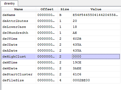
In FAT32 the index of the first cluster is obtained by combining the high-word deHighClust with the low-word deStartCluster in order to obtain a 32-bit index.
The problem is that the high-word has been zeroed. The actual value should be 0x0013. Seems this behavior is common on Microsoft operating systems as mentioned in this thread on Forensic Focus.
This means that only files with a cluster index equal or lower than 0xFFFF will be correctly pointed at. This makes another approach for FAT32 file recovery more appealing: instead of looking for deleted directly entries, one could directly look for cluster indexes with a value of 0 in the FAT and recognize the start of a file by matching signatures. Profiler offers an API to identify file signatures (although limited to the file formats it supports), so we could easily implement this logic. Another advantage of this approach is that it doesn't require a deleted file directory entry to work, increasing the possibility to recover deleted files. However, even that approach has certain disadvantages:
- Files which have no signature (like text files) or are not identified won't be recovered.
- The name of the files won't be recovered at all, unless they contain it themselves, but that's unlikely.
Disadvantages notwithstanding I think that if one had to choose between the two approaches the second one holds higher chances of success. So why then did I opt to do otherwise? Because I thought it would be nice to recover file names, even though only partially and delve a bit more in the format of FAT32. The blunt approach could be generalized more and requires less FAT knowledge.
However, the surely best approach is to combine both systems in order to maximize chances of recovery at the cost of duplicates. But this is just a demonstration, so let's keep it relatively simple and let's go back to the problem at hand: the incomplete start cluster index.
Recovering files only from lower parts of the disk isn't really good enough. We could try to recover the high-word of the index from adjacent directory entries of existing files. For instance, let's take a look at the deleted directory entry:
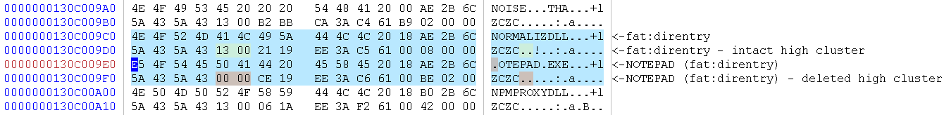
As you can see, the directory entry above the deleted one represents a valid file entry and contains an intact high-word we could use to repair our index. Please remember that this technique is just something I came up with and offers no guarantee whatsoever. In fact, it only works under certain conditions:
- The cluster containing the deleted entry must also contain a valid file directory entry.
- The FAT can't be heavily fragmented, otherwise the retrieved high-word might not be correct.
Still I think it's interesting and while it might not always be successful in automatic mode, it can be helpful when trying a manual recovery.
This is how the code to recover partial cluster indexes might look like:
def recoverClusterHighWord(fi, offs):
    cluster_start = offs - (offs % fi.bytes_per_clust)
    deloffs = offs - (offs % 0x20)
    nbefore = (deloffs - cluster_start) // 0x20
    nafter = (fi.bytes_per_clust - (deloffs - cluster_start)) // 0x20 - 1
    b = fi.obj.ToBuffer(deloffs + 0x20, Bufferize_BackAndForth)
    b.setBufferSize(fi.bytes_per_clust * 2)
    de_before = None
    de_after = None
    try:
        # try to find a valid entry before
        if nbefore > 0:
            for x in range(nbefore):
                b.setOffset(b.getOffset() - 0x40)
                # it can't be a deleted entry
                if b.u8() == 0xE5:
                    continue
                de = getDirEntryData(b)
                if validateFileDirectoryEntry(fi, de):
                    de_before = de
                    break
        # try to find a valid entry after
        if nafter > 0 and de_before == None:
            b.setOffset(deloffs + 0x20)
            for x in range(nafter):
                # it can't be a deleted entry
                if b.u8() == 0xE5:
                    continue
                de = getDirEntryData(b)
                if validateFileDirectoryEntry(fi, de):
                    de_after = de
                    break
    except:
        pass
    # return the high-word if any
    if de_before != None:
        return de_before.high_clust
    if de_after != None:
        return de_after.high_clust
    return 0
It tries to find a valid file directory entry before and after the deleted entry, remaining in the same cluster. Now we can write a small function to recover the file content.
# dump the content of a deleted file using the FAT
def dumpDeletedFileContent(fi, f, start_cluster, file_size):
    while file_size > 0:
        offs = clusterToOffset(fi, start_cluster)
        data = fi.obj.Read(offs, fi.bytes_per_clust)
        if file_size < fi.bytes_per_clust:
            data = data[:file_size]
        f.write(data)
        # next
        file_size = file_size - min(file_size, fi.bytes_per_clust)
        # find next cluster
        while True:
            start_cluster = start_cluster + 1
            idx_offs = start_cluster * 4 + fi.fat_offs
            idx, ok = fi.obj.ReadUInt32(idx_offs)
            if ok == False:
                return False
            if idx == 0:
                break
    return True
All the pieces are there, it's time to bring them together.
Create a recovery tool
With the recently introduced logic provider extensions, it's possible to create every kind of easy-to-use custom utility. Until now we have seen useful pieces of code, but using them as provided is neither user-friendly nor practical. Wrapping them up in a nice graphical utility is much better.
What follows is the source code or at least part of it: I have omitted those parts which haven't significantly changed. You can download the full source code from here.
Here's the cfg entry:
[FAT32Recovery]
label = FAT32 file recovery utility
descr = Recover files from a FAT32 partition or drive.
file = fat32_recovery.py
init = FAT32Recovery_init
And the Python code:
class RecoverySystem(LocalSystem):

    def __init__(self):
        LocalSystem.__init__(self)
        self.ctx = proCoreContext()
        self.partition = None
        self.current_partition = 0
        self.fi = None
        self.counter = 0

    def wasAborted(self):
        Pro.UI.proProcessEvents(1)
        return self.ctx.wasAborted()

    def nextFile(self):
        fts = FileToScan()

        if self.partition == None:
            # get next partition
            while self.current_partition < 4:
                entryoffs = 0x1BE + (self.current_partition * 0x10)
                self.current_partition = self.current_partition + 1
                offs, ret = self.disk.ReadUInt32(entryoffs + 8)
                size, ret = self.disk.ReadUInt32(entryoffs + 12)
                if offs != 0 and size != 0:
                    cpartition = self.disk.GetStream()
                    cpartition.setRange(offs * 512, size * 512)
                    part = CFFObject()
                    part.Load(cpartition)
                    self.fi = setupFATData(part)
                    if self.fi != None:
                        self.fi.system = self
                        self.partition = part
                        self.next_entry = self.fi.data_offs
                        self.fi.ascii_names_conv = self.ascii_names_conv
                        self.fi.repair_start_clusters = self.repair_start_clusters
                        self.fi.max_file_size = self.max_file_size
                        break

        if self.partition != None:
            de = findDeletedFiles(self.fi, self.next_entry)
            if de != None:
                self.next_entry = de.offs + 0x20
                fname = "%08X" % self.counter
                f = open(self.dump_path + fname, "wb")
                if f == None:
                    ctx.msgBox(MsgErr, "Couldn't open file '" + fname + "'")
                    return fts
                dumpDeletedFileContent(self.fi, f, de.clust_idx, de.file_size)
                f.close()
                self.counter = self.counter + 1
                fts.setName(fname + "\\" + de.name)
                fts.setLocalName(self.dump_path + fname)
            else:
                self.partition = None

        return fts

def recoveryOptionsCallback(pe, id, ud):
    if id == Pro.UI.ProPropertyEditor.Notification_Close:
        path = pe.getValue(0)
        if len(path) == 0 or os.path.isdir(path) == False:
            errs = NTIntList()
            errs.append(0)
            pe.setErrors(errs)
            return False
    return True

def FAT32Recovery_init():
    ctx = Pro.UI.proContext()
    file_name = ctx.getOpenFileName("Select disk...")
    if len(file_name) == 0:
        return False

    cdisk = createContainerFromFile(file_name)
    if cdisk.isNull():
        ctx.msgBox(MsgWarn, "Couldn't open disk!")
        return False

    disk = CFFObject()
    disk.Load(cdisk)
    bsign = disk.Read(0x1FE, 2)
    if len(bsign) != 2 or bsign[0] != 0x55 or bsign[1] != 0xAA:
        ctx.msgBox(MsgWarn, "Invalid MBR!")
        return False

    dlgxml = """


"""
    opts = ctx.askParams(dlgxml, "FAT32RecoveryOptions", recoveryOptionsCallback, None)
    if opts.isEmpty():
        return False

    s = RecoverySystem()
    s.disk = disk
    s.dump_path = os.path.normpath(opts.value(0)) + os.sep
    s.ascii_names_conv = "strict" if opts.value(1) else "replace"
    s.repair_start_clusters = opts.value(2)
    if opts.value(3) != 0:
        s.max_file_size = opts.value(3) * 1024 * 1024
    proCoreContext().setSystem(s)
    return True
When the tool is activated it will ask for the disk file to be selected, then it will show an options dialog.
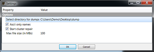
In our case we can select the option 'Ascii only names' to exclude false positives.
The options dialog asks for a directory to save the recovered files. In the future it will be possible to save volatile files in the temporary directory created for the report, but since it's not yet possible, it's the responsibility of the user to delete the recovered files if he wants to.
The end results of the recovery operation:
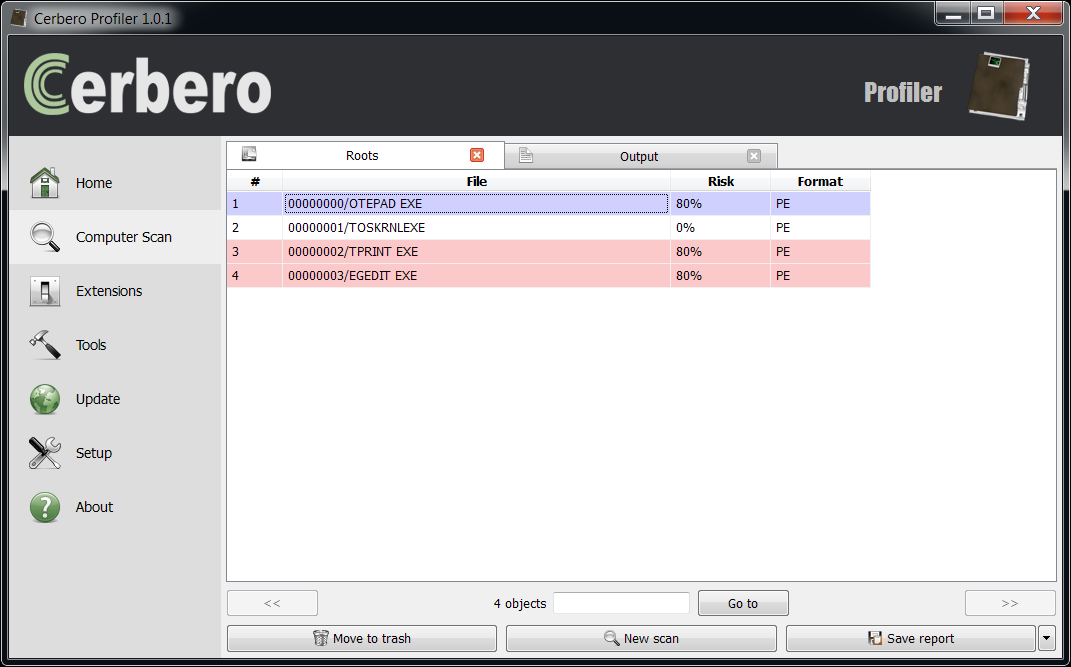
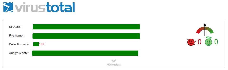
All four deleted files have been successfully recovered.
Three executables are marked as risky because intrinsic risk is enabled and only 'ntoskrnl.exe' contains a valid digital certificate.
Conclusions
I'd like to remind you that this utility hasn't been tested on disks other than on the one I've created for the post and, as already mentioned, it doesn't even implement the best method to recover files from a FAT32, which is to use a signature based approach. It's possible that in the future we'll improve the script and include it in an update.
The purpose of this post was to show some of the many things which can be done with Profiler. I used only Profiler for the entire job: from analysis to code development (I even wrote the entire Python code with it). And finally to demonstrate how a utility with commercial value like the one presented could be written in under 300 lines of Python code (counting comments and new-lines).
The advantages of using the Profiler SDK are many. Among them:
- It hugely simplifies the analysis of files. In fact, I used only two external Python functions: one to check the existence of a directory and one to normalize the path string.
- It helps building a fast robust product.
- It offers a graphical analysis experience to the user with none or little effort.
- It gives the user the benefit of all the other features and extension offered by Profiler.
To better explain what is meant by the last point, let's take the current example. Thanks to the huge amount of formats supported by Profiler, it will be easy for the user to validate the recovered files.
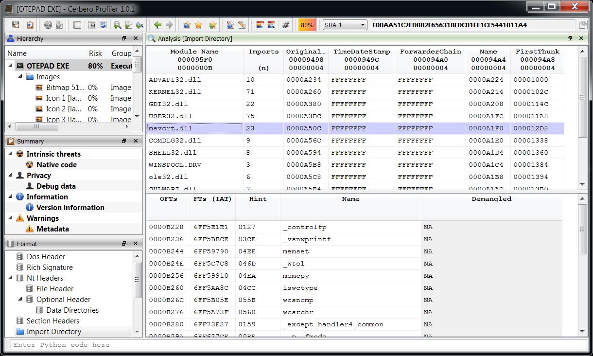
In the case of Portable Executables it's extremely easy because of the presence of digital certificates, checksums and data structures. But even with other files it's easy, because Profiler may detect errors in the format or unused ranges.
I hope you enjoyed this post!
P.S. You can download the complete source code and related files from here.
References
- File System Forensic Analysis - Brian Carrier
- Understanding FAT32 Filesystems - Paul Stoffregen
- Official documentation - Microsoft
- File Allocation Table - Wikipedia
- Master boot record - Wikipedia