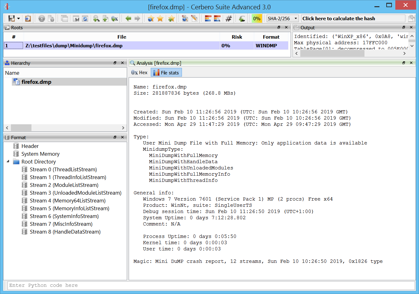
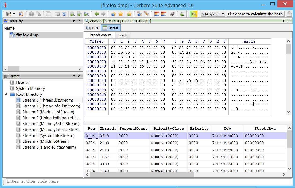
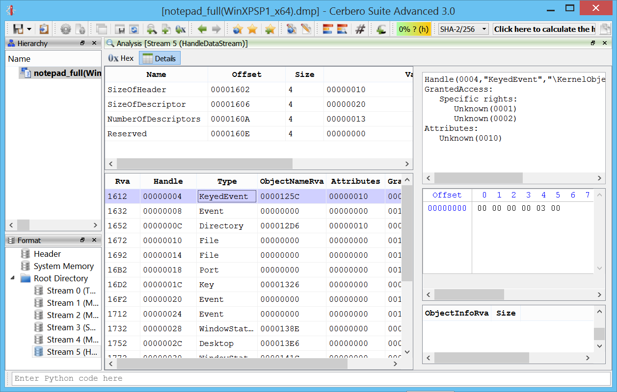
Getting close to the release date of the 3.0 version of Cerbero Suite, it’s time to announce the main feature of the advanced edition: an interactive disassembler for x86/x64.
The initial intent was to enable our users to inspect code in memory dumps as well as shellcode. Today we have very advanced disassemblers such as IDA and Ghidra and it wouldn’t have made sense to try and mimic one of these tools. That’s why I approached the design of the disassembler also considering how Cerbero Suite is being used by our customers.
Cerbero Suite is heavily used as a tool for initial triage of files and that’s why I wanted its disassembler to reflect this nature. I remembered the good old days using W32Dasm and took inspiration from that. Of course, W32Dasm wouldn’t be able to cope with the complexity of today’s world and a 1:1 transposition wouldn’t work.
That’s why in the design of Carbon I tried to combine the immediacy of a tool such as W32Dasm with the flexibility of a more advanced one.
So let’s start with presenting a list of features:
Flat disassembly view
The Carbon disassembler comes with a flat disasm view showing all the instructions in a file. I don’t exclude it will feature a graph view one day as well, but it’s not a priority.
Recursive disassembly
A recursive disassembler is necessary to tackle cases in which the code is interrupted by data. Carbon will try to do its best to disassemble in a short period of time, while still performing basic analysis.
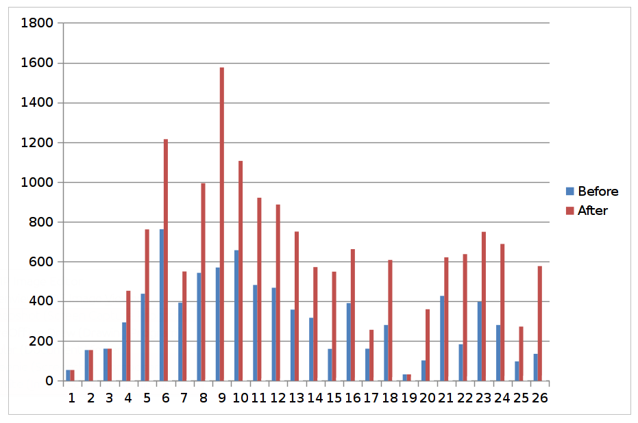
Speed
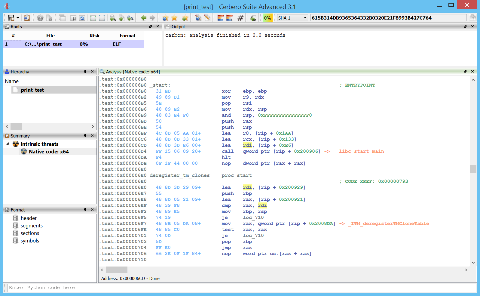
Carbon is multi-thread and seems to handle large files quite fast. This is very useful for the initial triage of a file.
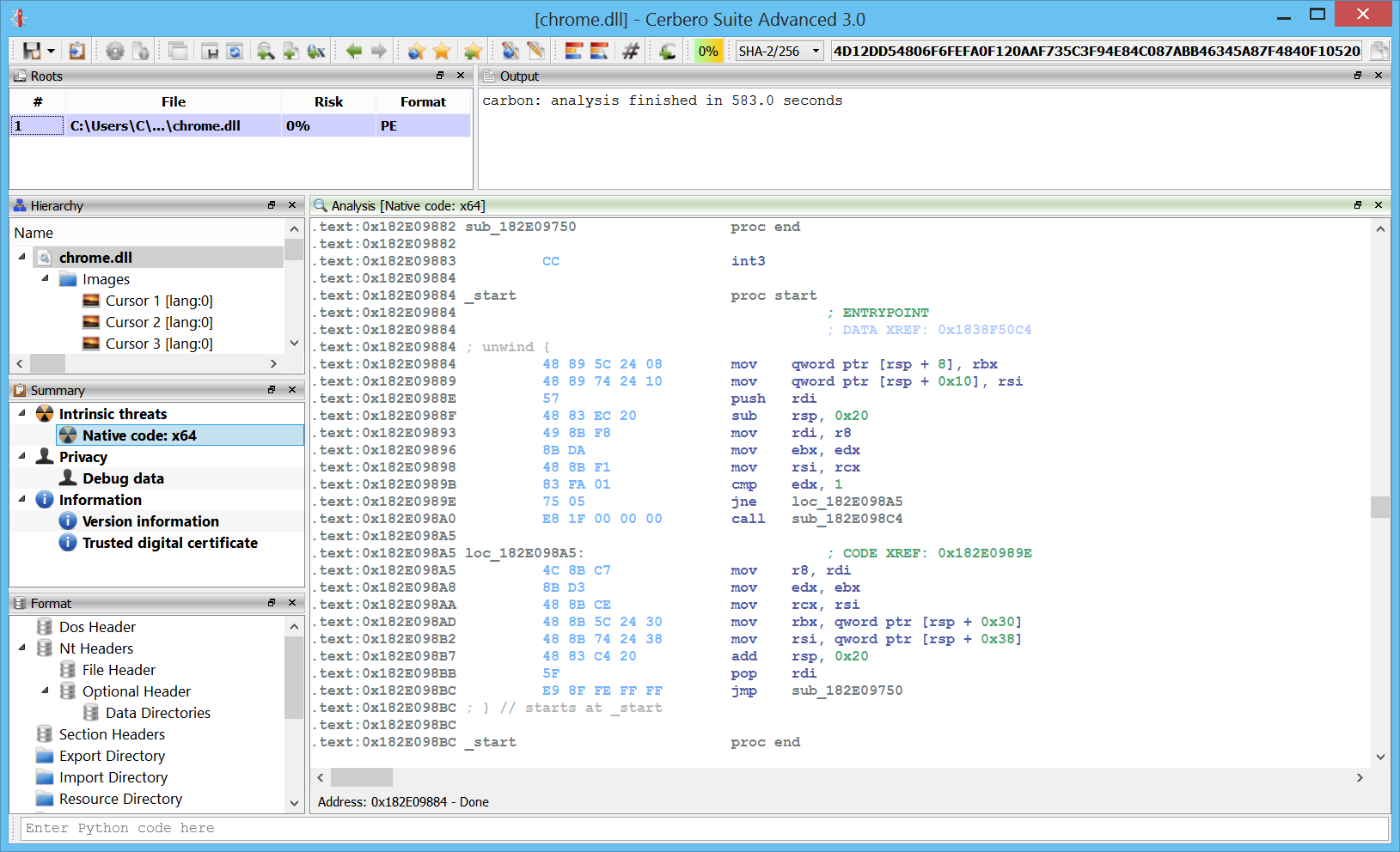
Here we can see the analysis on a 60 MB chrome DLL performed in about ten minutes. And this while running in a virtual machine.
The challenge in the future will be to maintain speed while adding even more analysis passages.
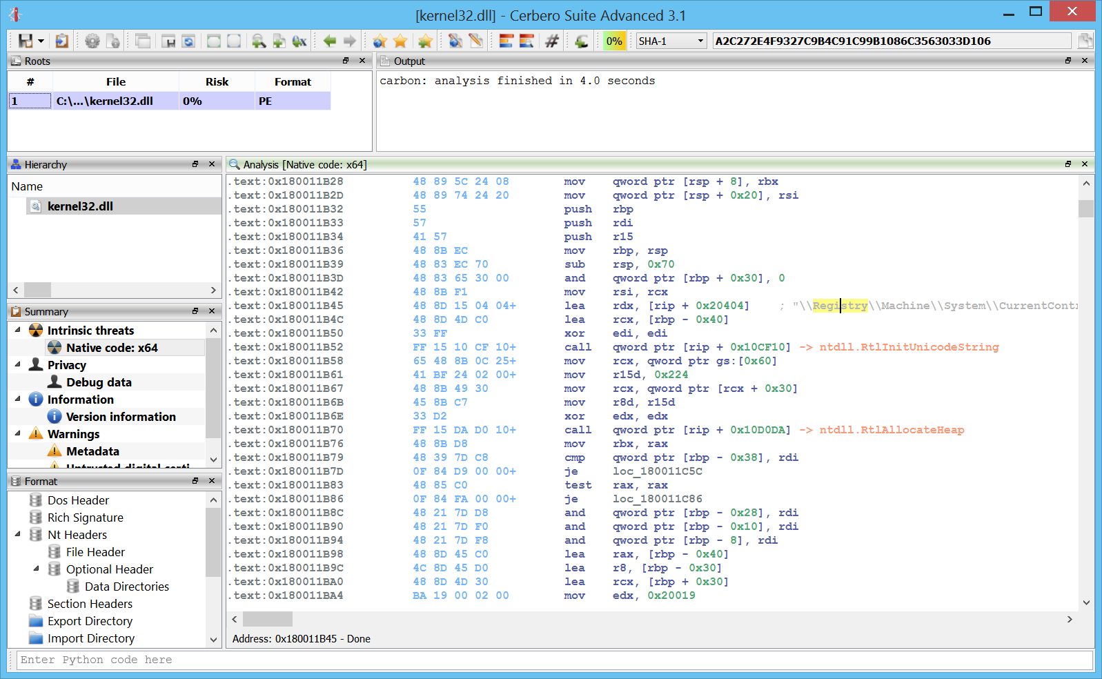
x86/x64 support
Carbon supports both x86 and x64 code. More architectures will be added in the future.
In fact, the design of Carbon will permit to mix architectures in the same disassembly view.
Unlimited databases
A single project in Cerbero can contain unlimited Carbon databases. This means if you’re analyzing a Zip file with 10 executable files, then every one of these files can have its own database.
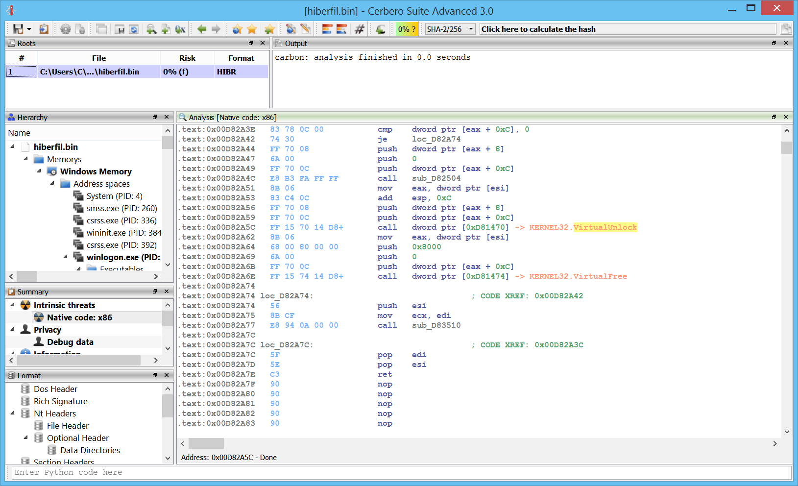
Not only that: a single file can have multiple databases, just click on the Carbon toolbar button or press “Ctrl+Alt+C” to add a new Carbon database.
And if you’re not satisfied with an analysis, it’s not an issue: you can easily delete it by right-clicking on the related Summary entry or by selecting it and pressing “Del”.
Scripting
As most of the functionality of Cerbero Suite is exposed to Python, this is true for Carbon as well. Most of the code of Carbon, including its database, is exposed to Python.
We can load and disassemble a file in a few lines of code.
    s = createContainerFromFile(a)
    obj = PEObject()
    obj.Load(s)

    c = Carbon()
    c.setObject(obj, True)
    if c.createDB(dbname) != CARBON_OK:
        print("error: couldn't create DB")
        return False
    if c.load() != CARBON_OK:
        print("error: couldn't load file")
        return False
    c.resumeAnalysis()
    # wait for the analysis to finish...
We can modify and explore every part of its internal database after the analysis has been completed, or we can create a view and show the disassembly:
    ctx = proContext()
    v = ctx.createView(ProView.Type_Carbon, "test")
    ctx.addView(v, True)
    v.setCarbon(c)
The internal database uses SQLite, making it easy to explore and modify it even without using the SDK.
Python loaders
I took early on the decision of writing all file loaders in Python. While this may make the loading itself of the file a little slower (although not that much), it provides enormous flexibility by allowing users to customize the loaders and adding functionality. Also adding new file loaders is extremely simple.
The whole loader for PE files is about 350 lines of code. And here is the loader for raw files:
from Pro.Carbon import *

class RawLoader(CarbonLoader):

    def __init__(self):
        super(RawLoader, self).__init__()

    def load(self):
        # get parameters
        p = self.carbon().getParameters()
        try:
            arch = int(p.value("arch", str(CarbonType_I_x86)), 16)
        except:
            print("carbon error: invalid arch")
            arch = CarbonType_I_x86
        try:
            base = int(p.value("base", "0"), 16)
        except:
            print("carbon error: invalid base address")
            base = 0
        # load
        db = self.carbon().getDB()
        obj = self.carbon().getObject()
        # add region
        e = caRegion()
        e.def_type_id = arch
        e.flags = caRegion.READ | caRegion.WRITE | caRegion.EXEC
        e.start = base
        e.end = e.start + obj.GetSize()
        e.offset = 0
        db.addRegion(e)
        # don't disassemble automatically
        db.setState(caMain.FINISHED)
        return CARBON_OK

def newRawLoader():
    return RawLoader()
Once you’re familiar with the SDK, it’s quite easy to add new loaders.
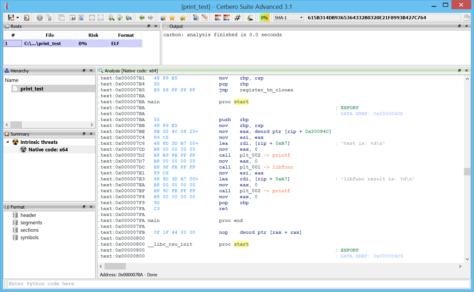
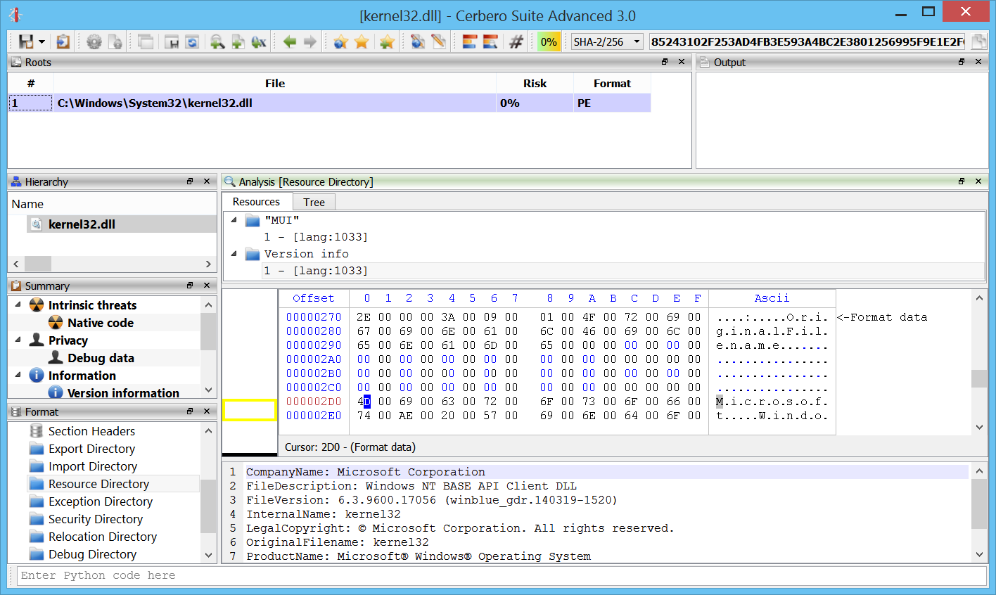
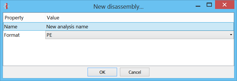
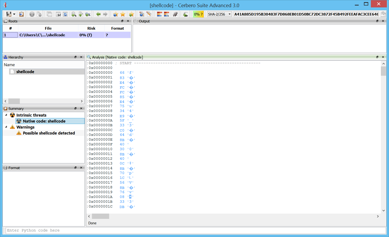
Raw / PE loader
Initial file support comes for PE and raw files.
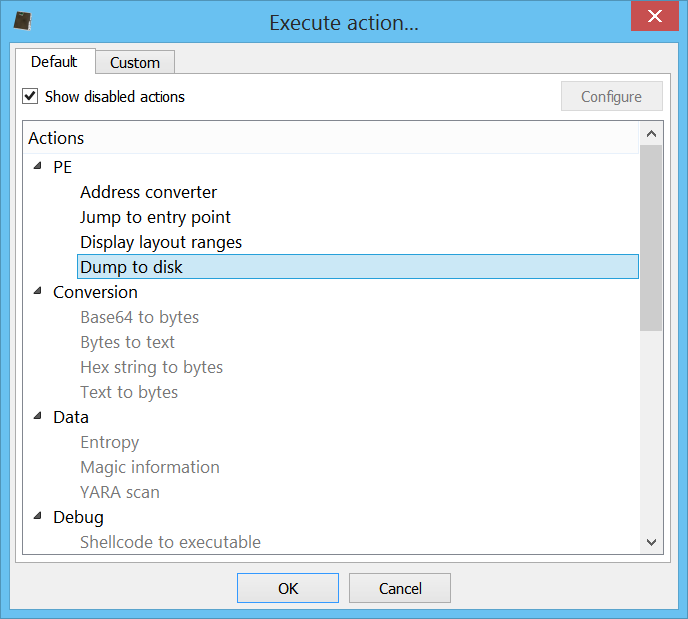
This, for instance, is some disassembled shellcode.
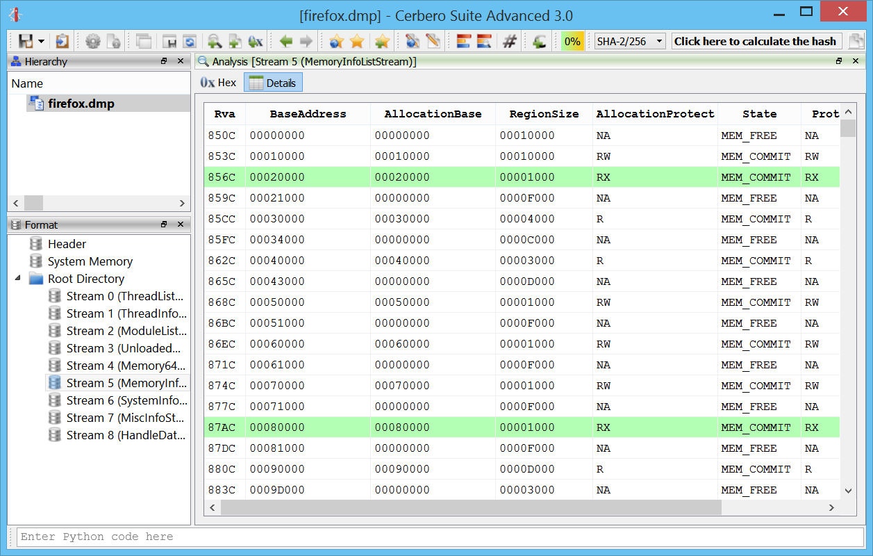
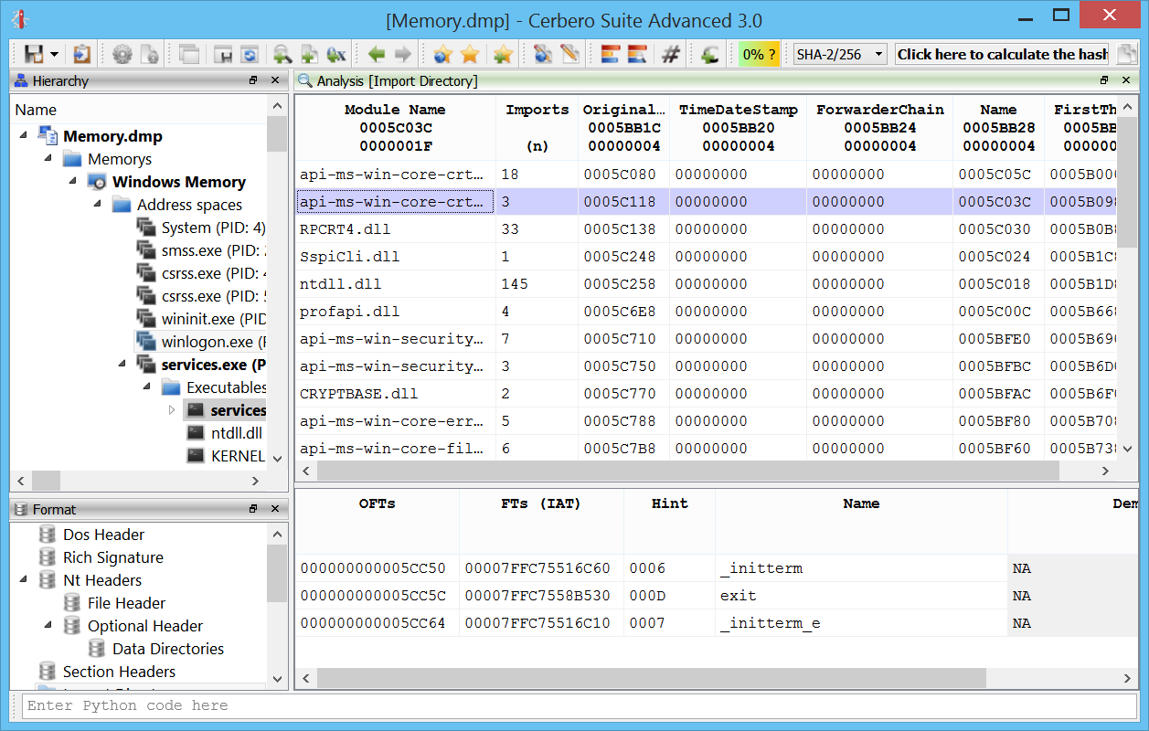
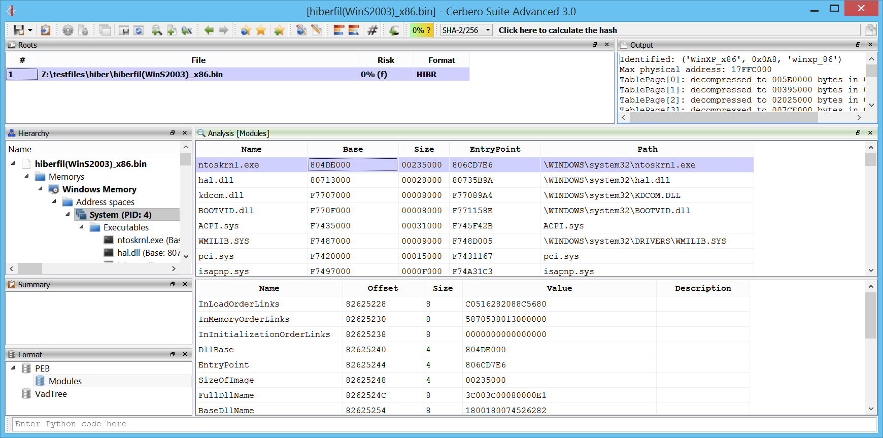
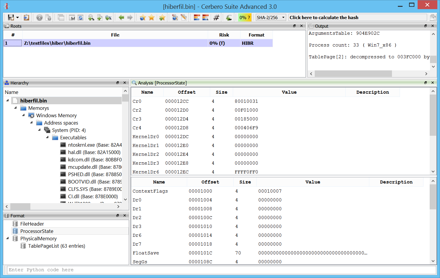
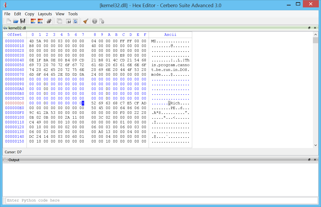
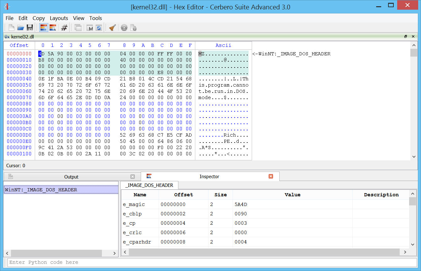
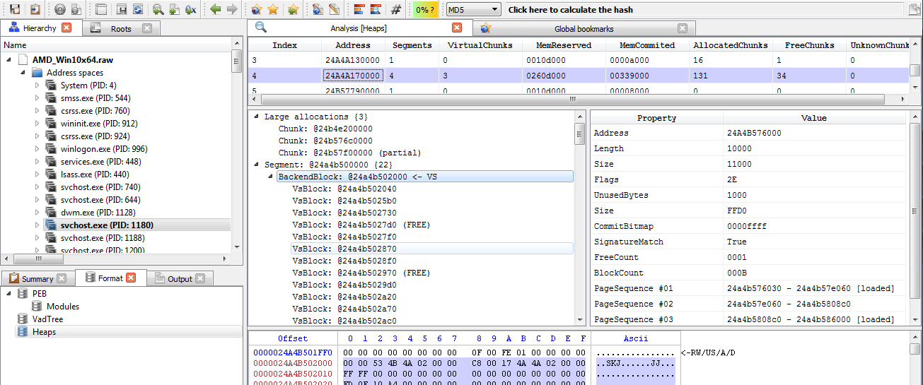
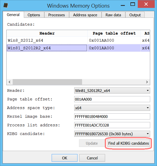
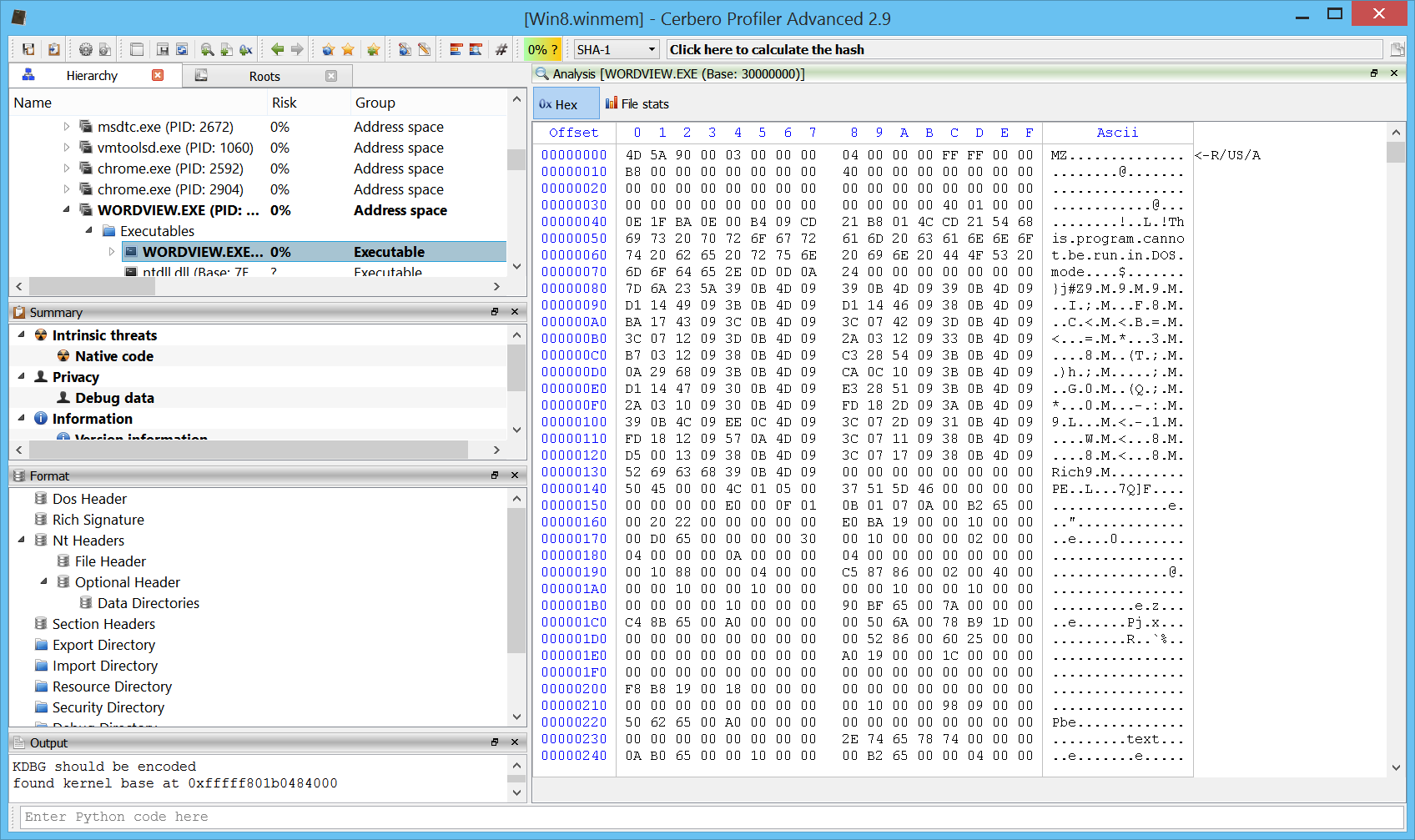
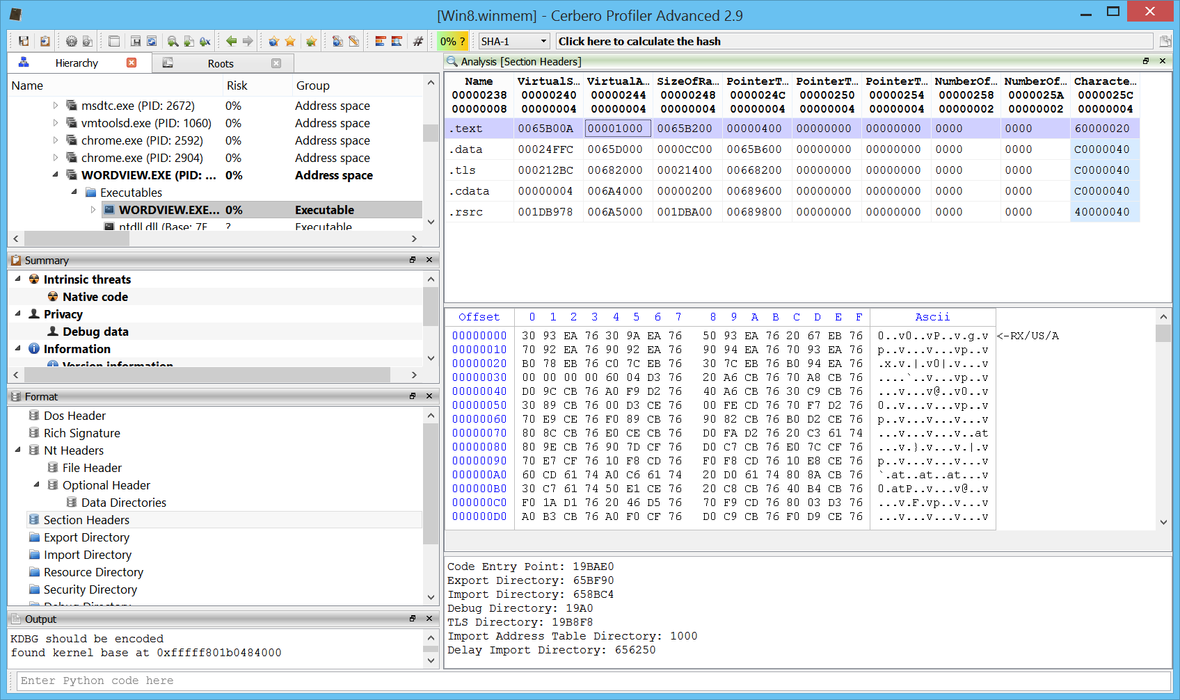
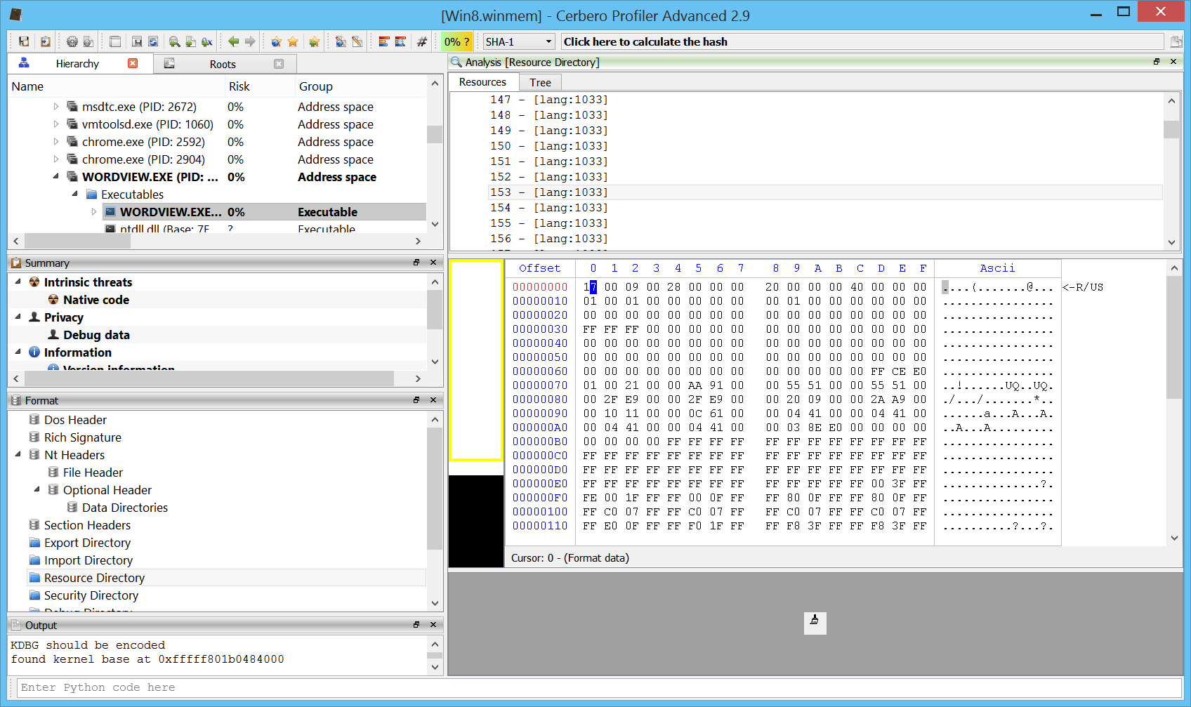
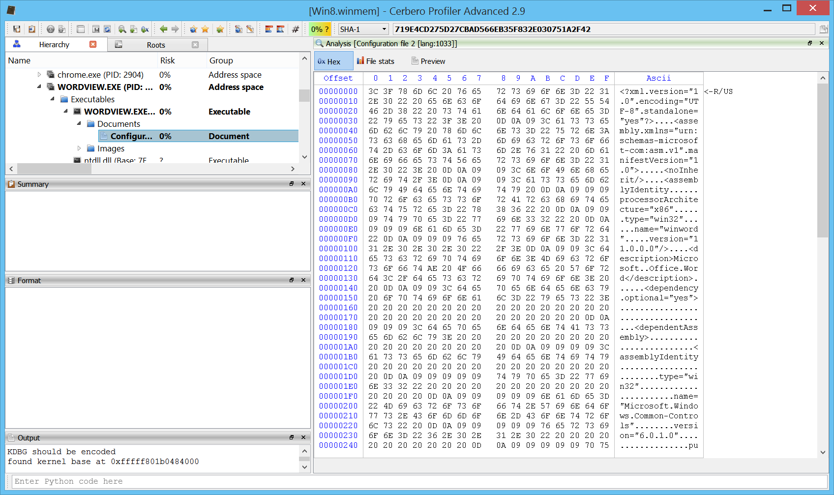
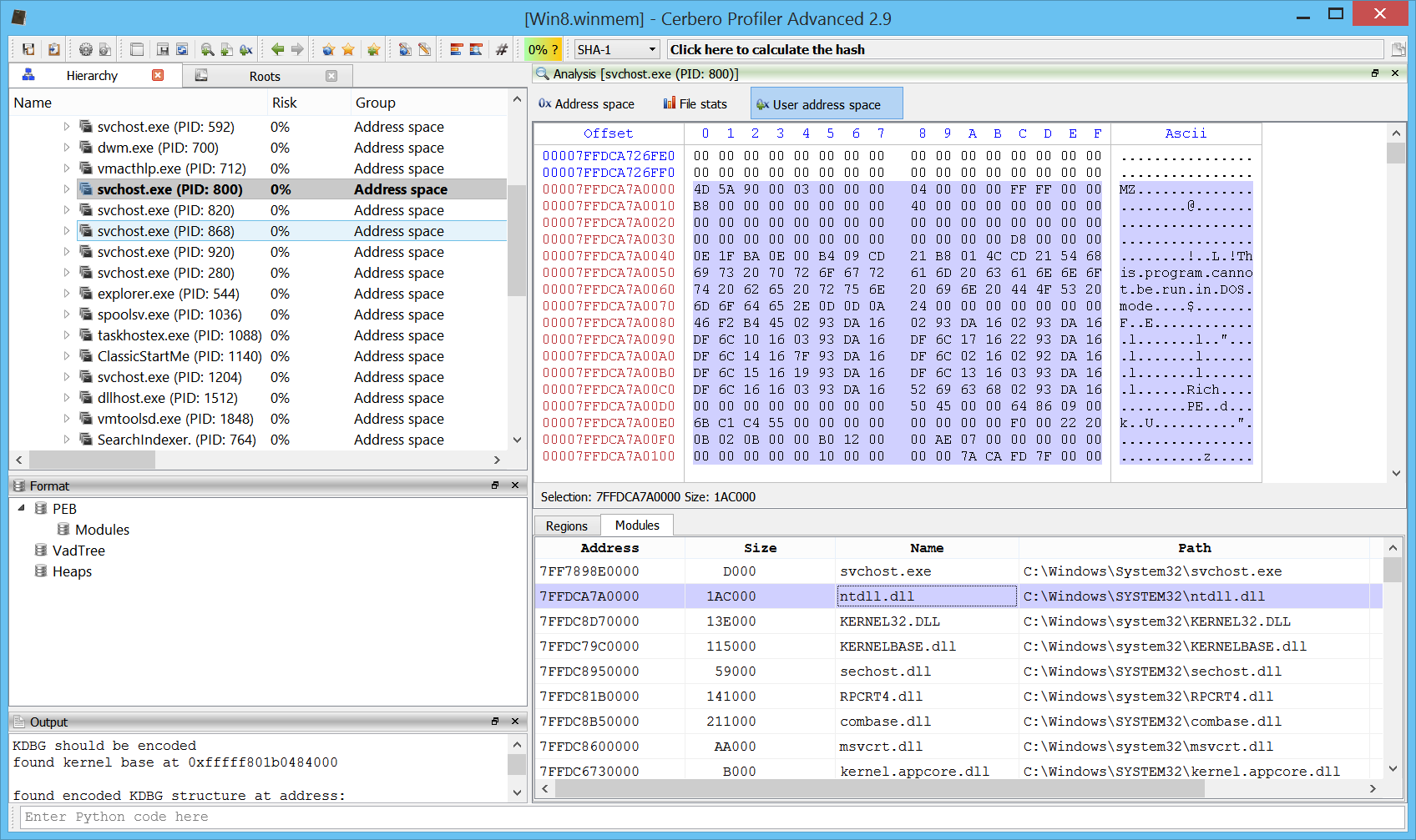
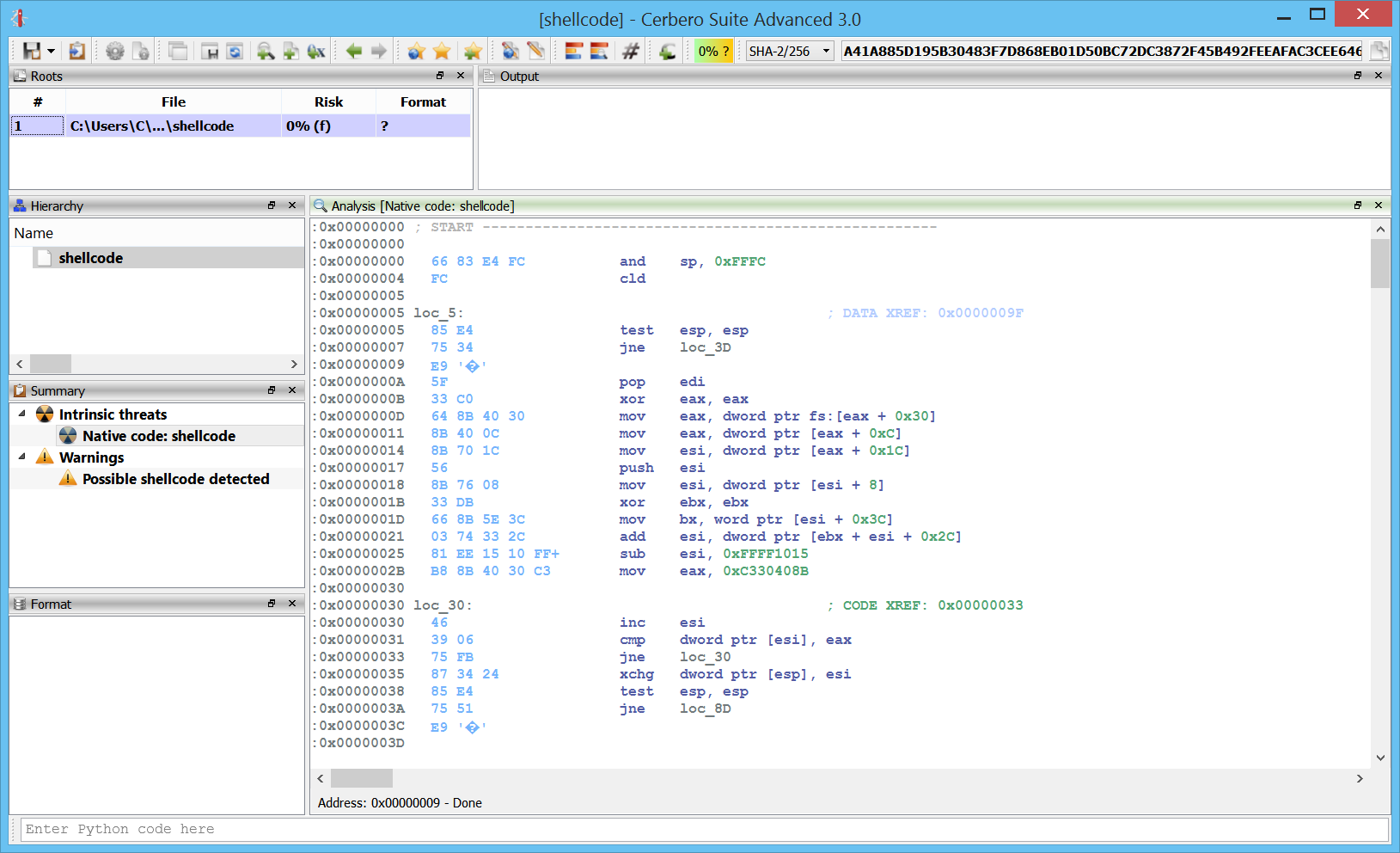
In memory PEs
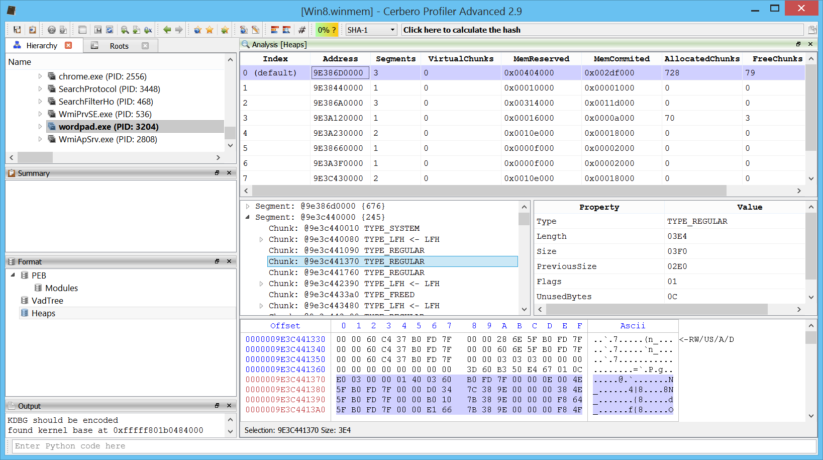
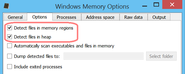
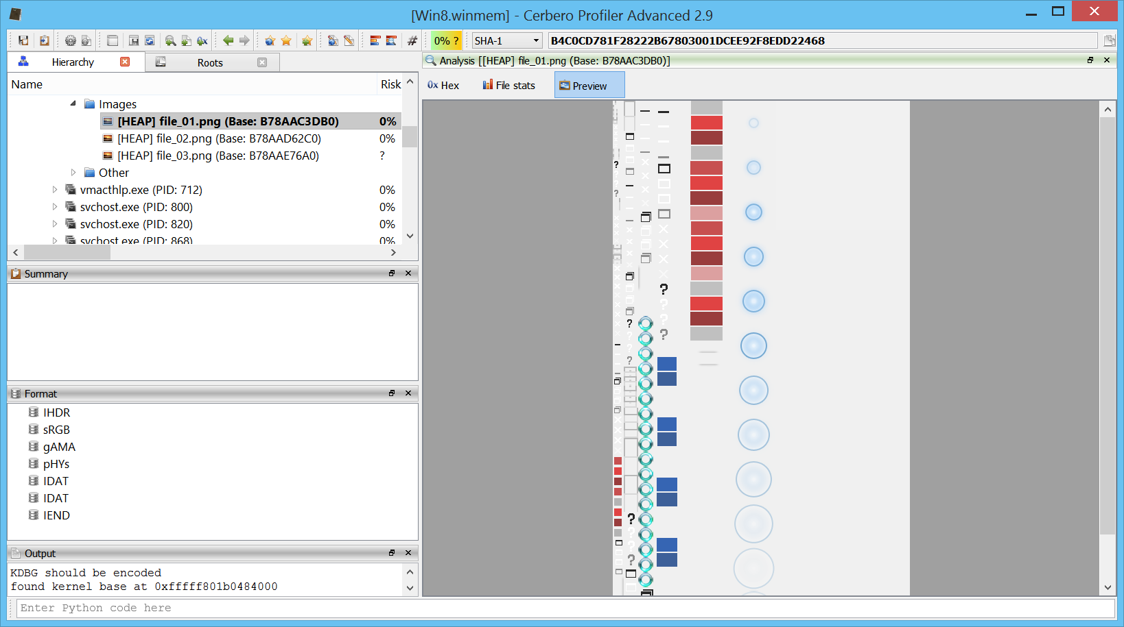
One of the main cool features is the capability to analyze in-memory PE files.
Here is the code of an in-memory PE:
Of course, the disassembly is limited to memory pages which haven’t been paged out, so there might be some gaps.
We haven’t played yet much with this feature and its functionality will be extended with upcoming releases.
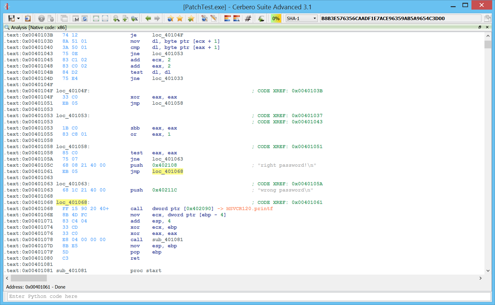
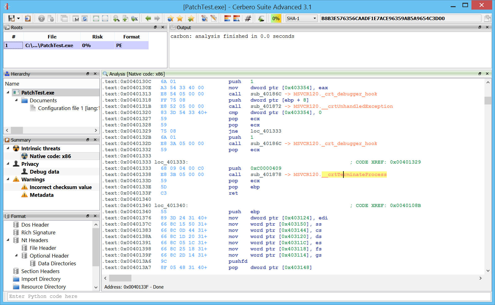
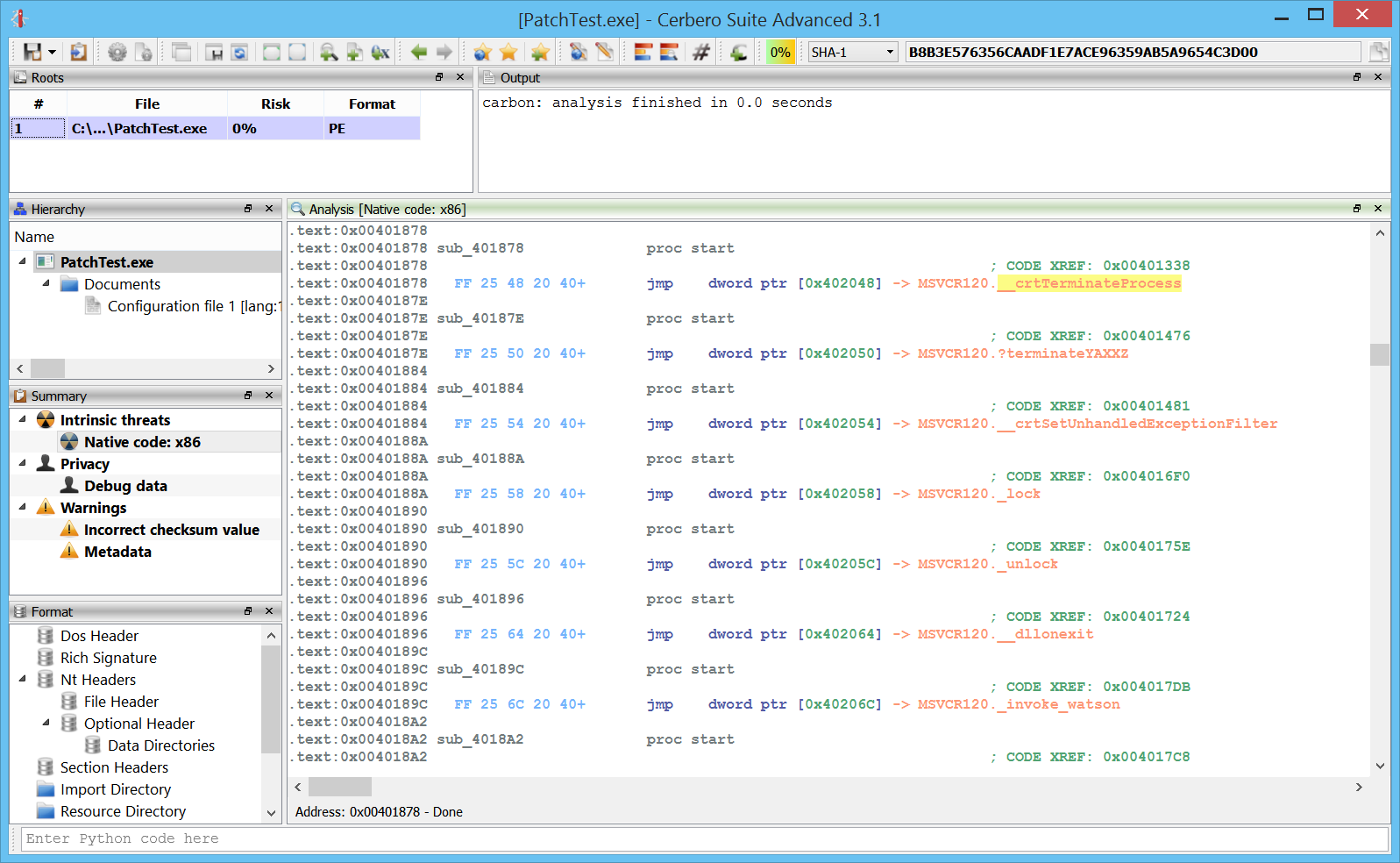
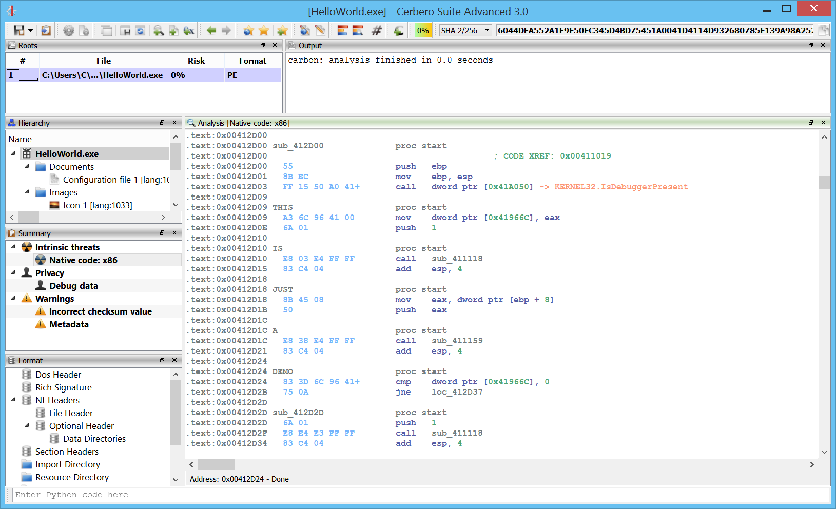
Cross references
Of course, no decent disassembler can lack cross references:
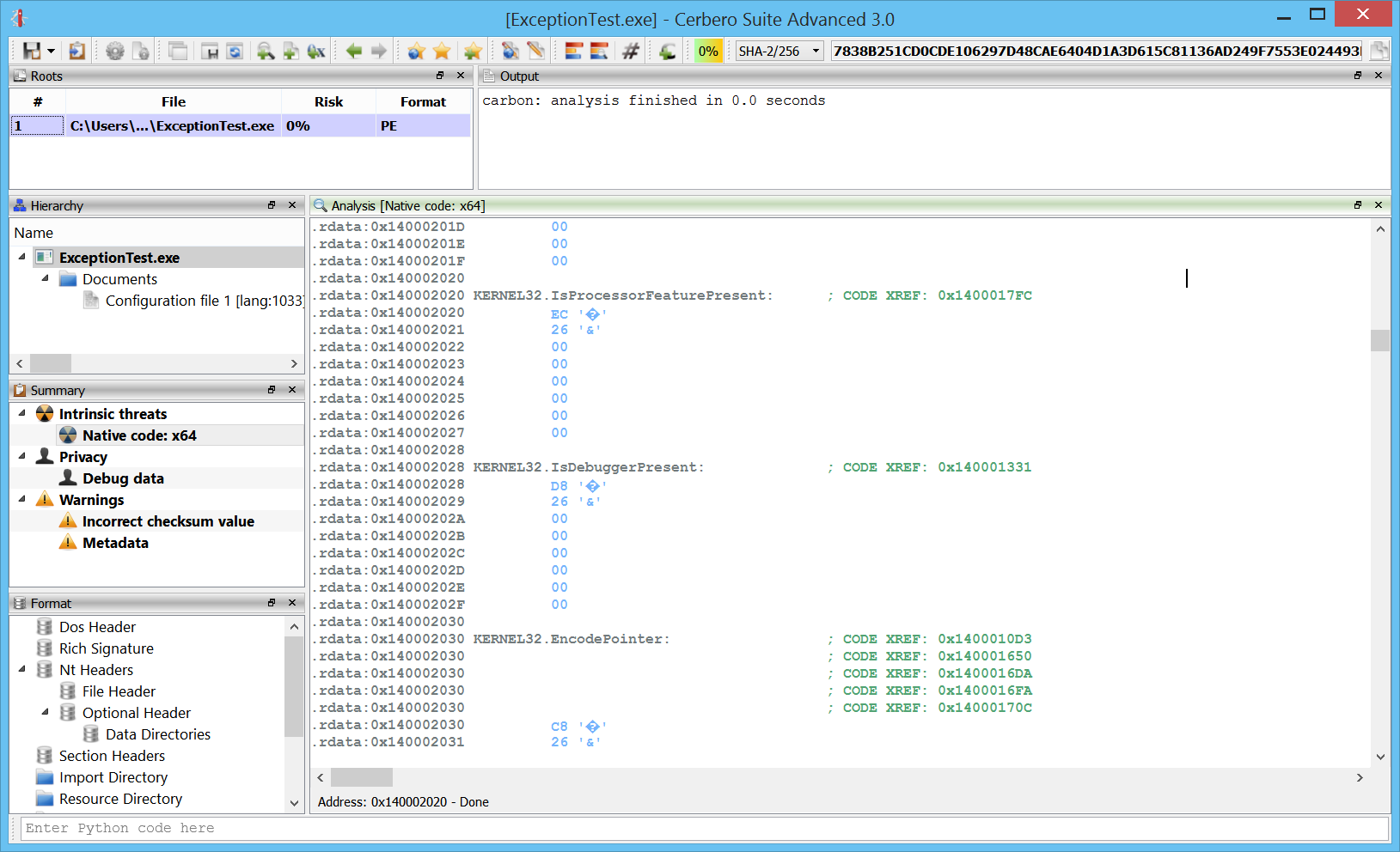
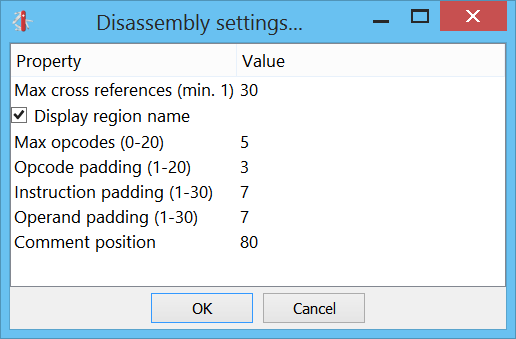
We can also choose how many cross references we want to see from the settings:
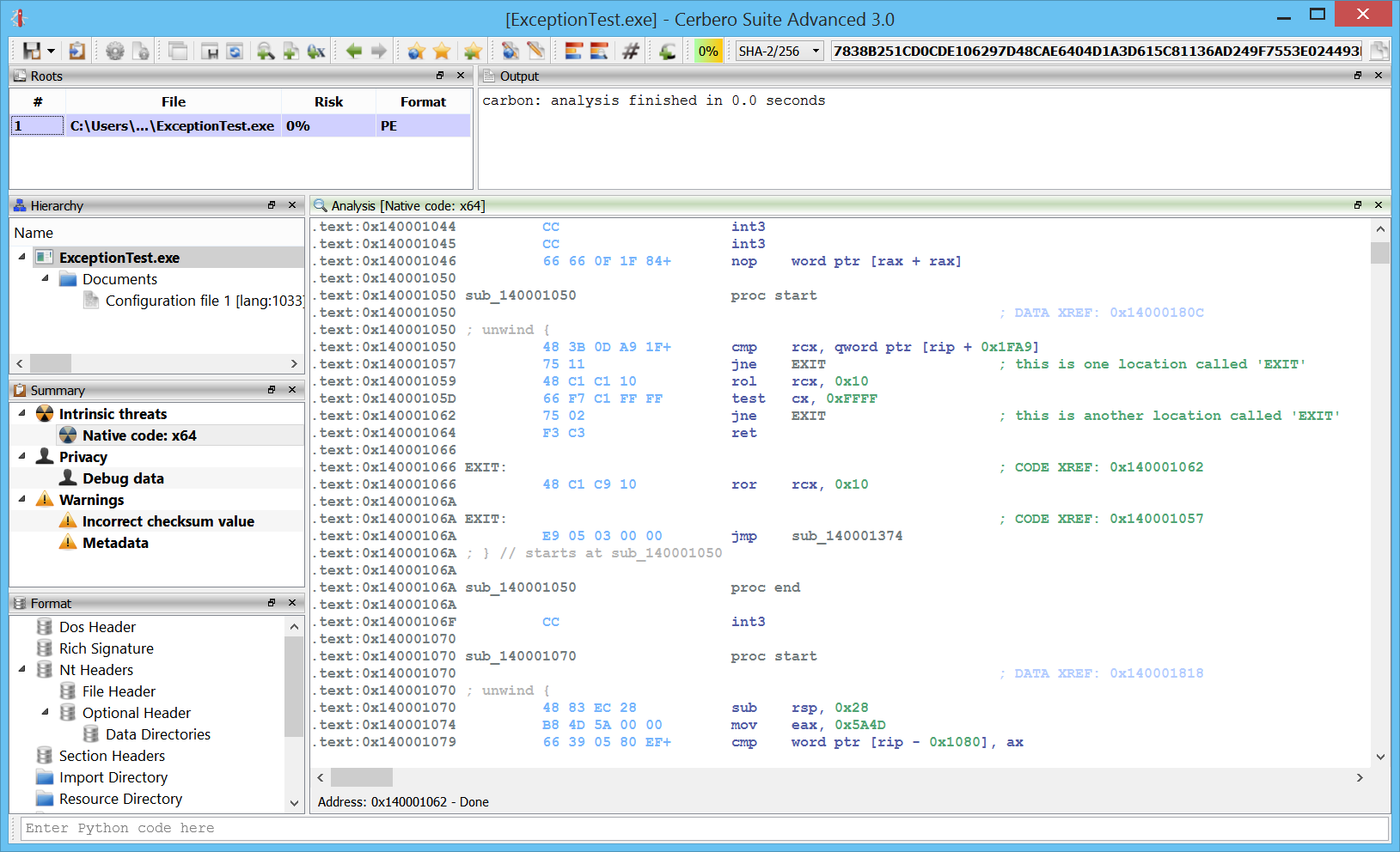
Renaming
We can name and rename any location or function in the code. Duplicates are allowed. Any why shouldn’t they? We could have more than one method with “jmp ERROR” instances, even if the ERROR doesn’t point to the same location.
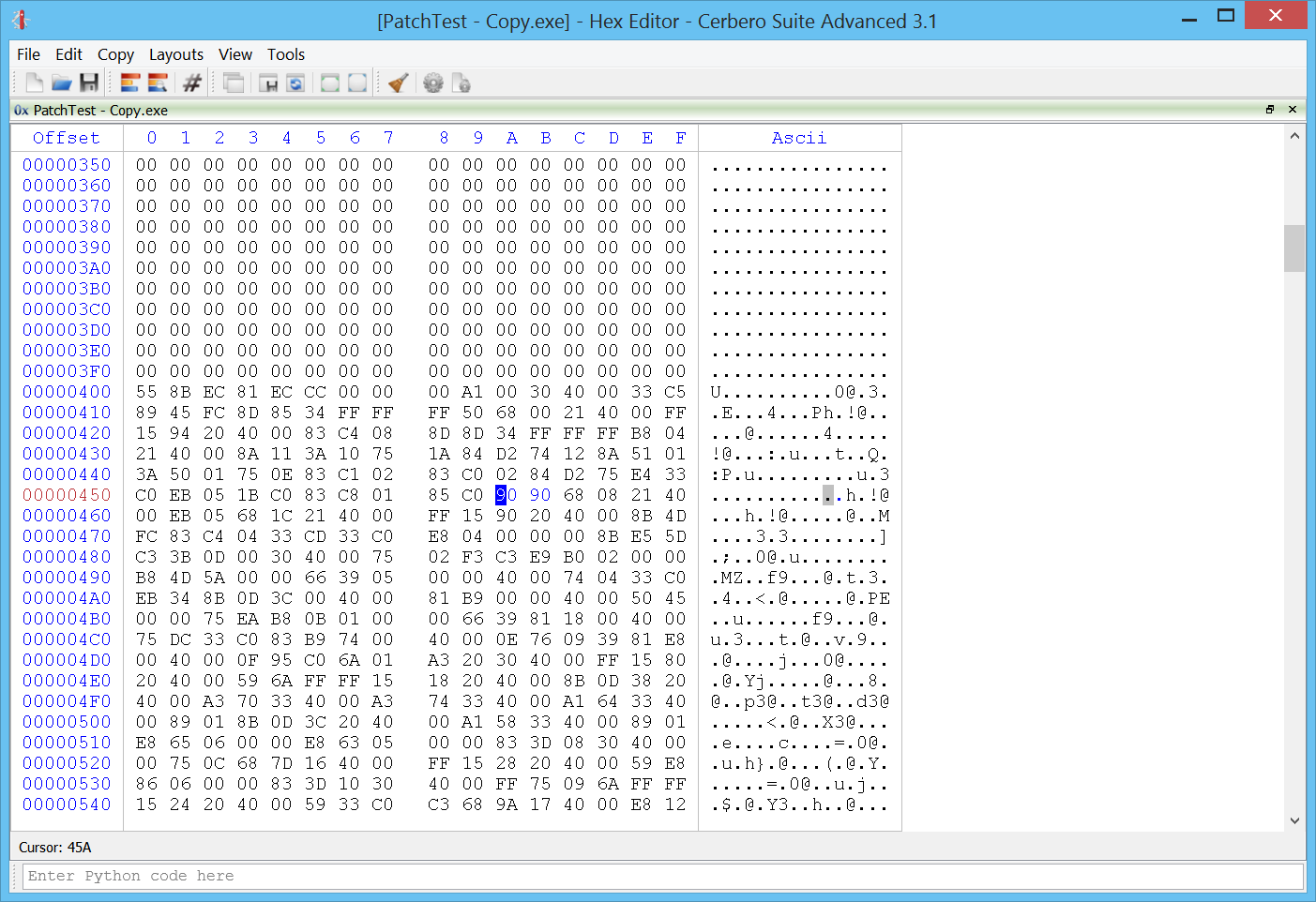
Make code/undefine
We can transform undefined data to code by pressing “C” or, conversely, transform code to undefined data pressing “U”.
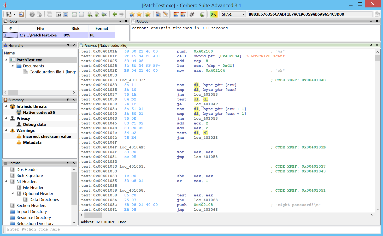
Here we add a new Carbon database to a shellcode. As you can see it’s all undefined data initially:
After pressing “C” at the first byte, we get some initial instructions:
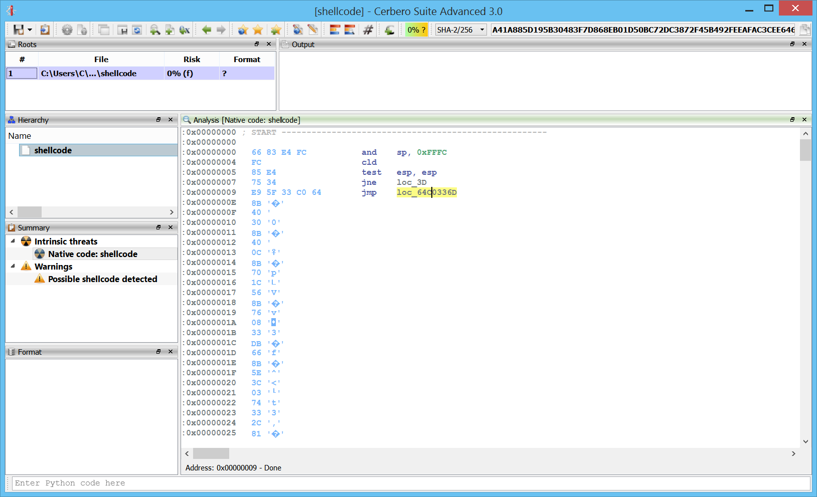
However, as we can see, the highlighted jump is invalid. By following the “jne” before of the “jmp” we can see that we actually jump in a byte after the “jmp” instruction. So what we do is to press “U” on the “jmp” and then press “C” on the byte at address 0xA.
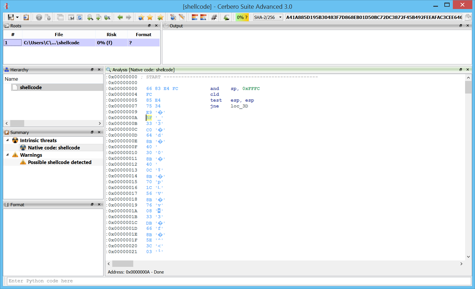
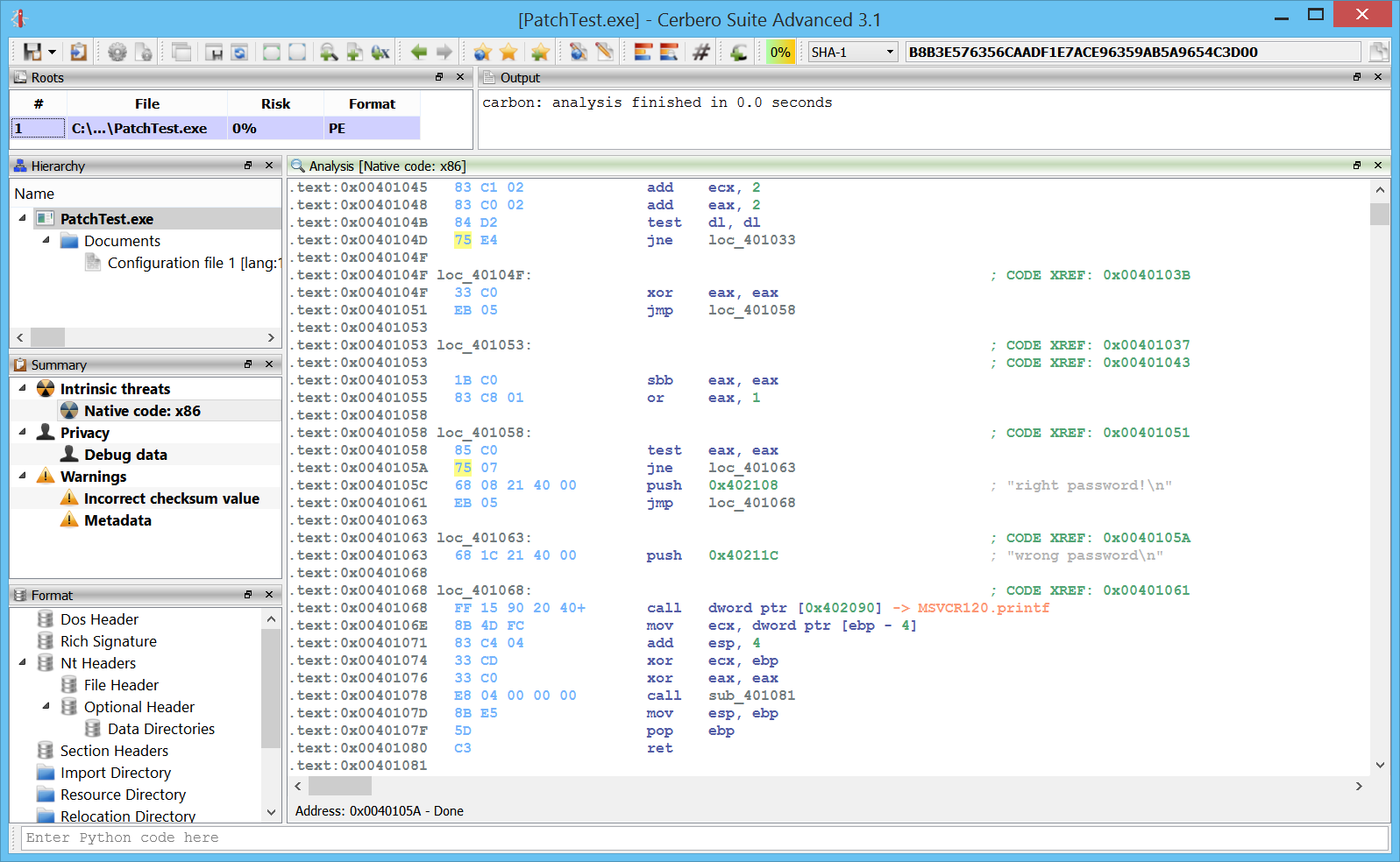
After pressing “C” again at 0xA:
Now we can properly analyze the shellcode.
Functions
We can easily define and undefine functions wherever we want.
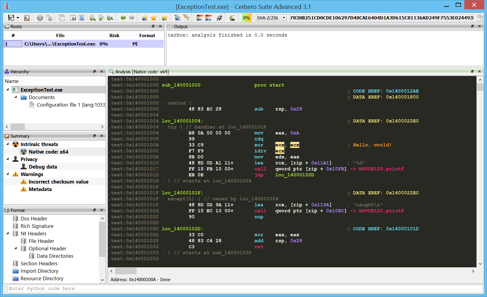
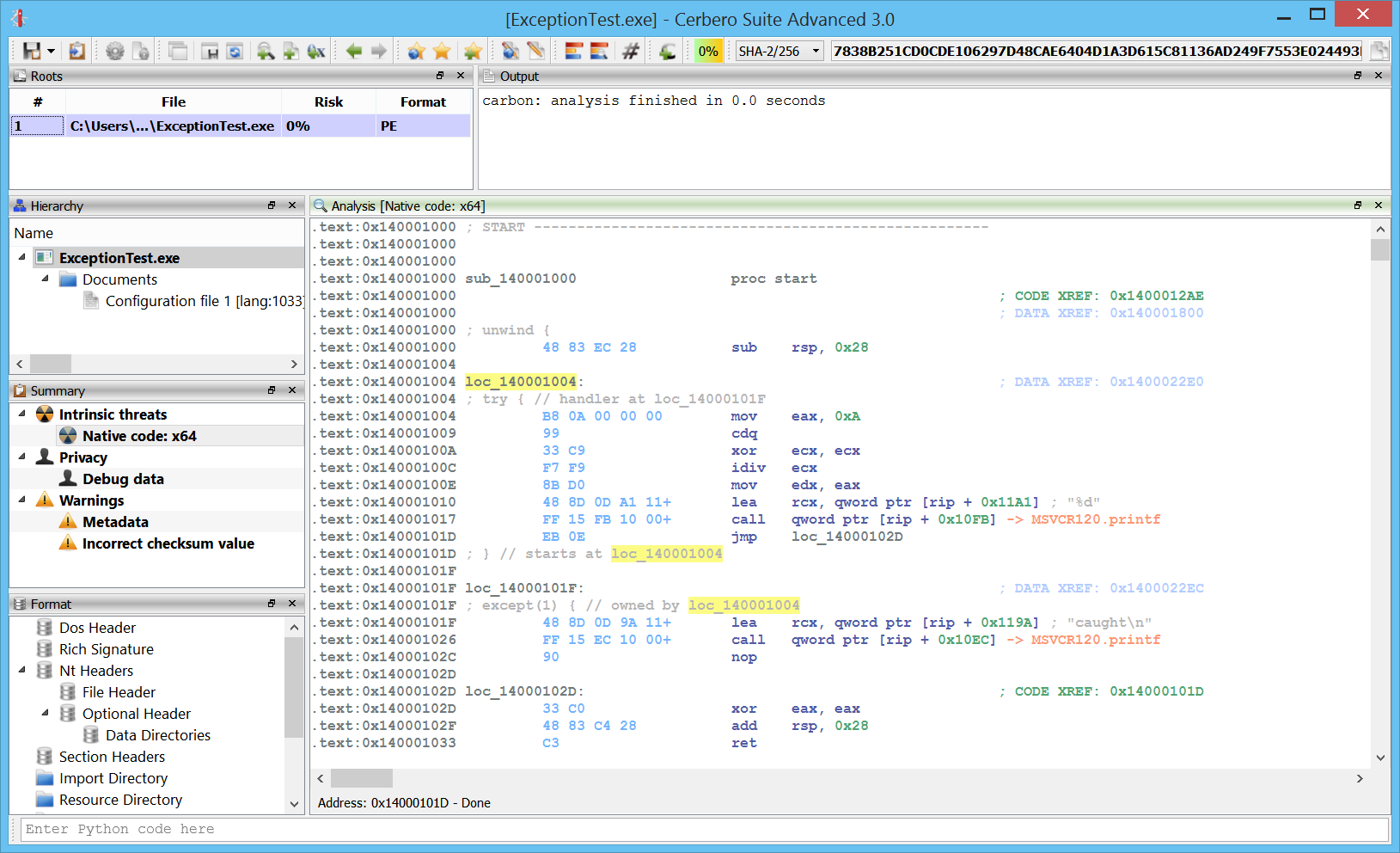
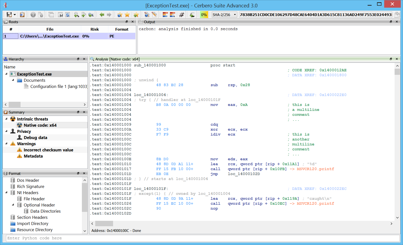
Exceptions
x64 exceptions are already supported.
Comments
One of the most essential features is the capability to add comments.
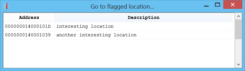
Flagged locations
You can also flag locations by pressing “Alt+M” or jump to a flagged location via “Ctrl+M”.
Lists
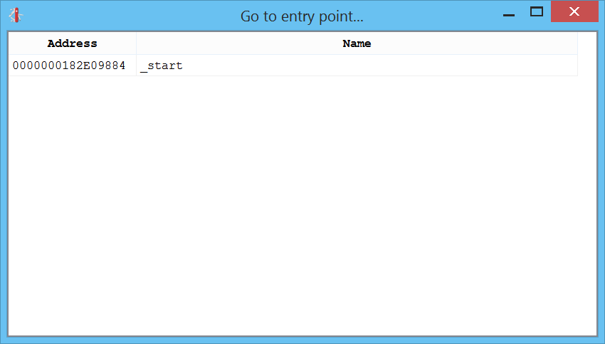
The shortcuts going from “Ctrl+1” to “Ctrl+4” present you various lists of things in the disassembly which you can go to.
Ctrl+1 shows the list of entry-points:
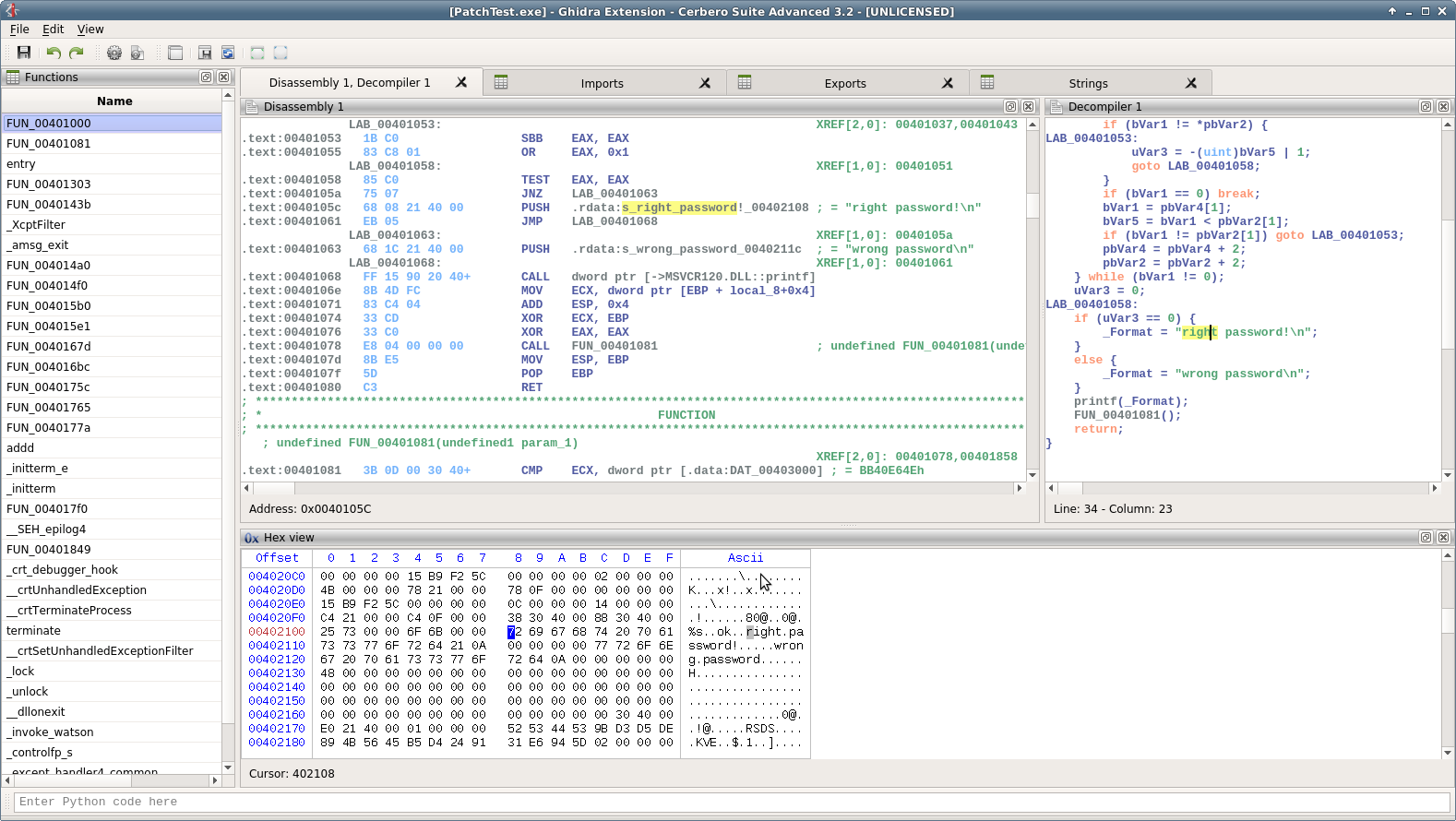
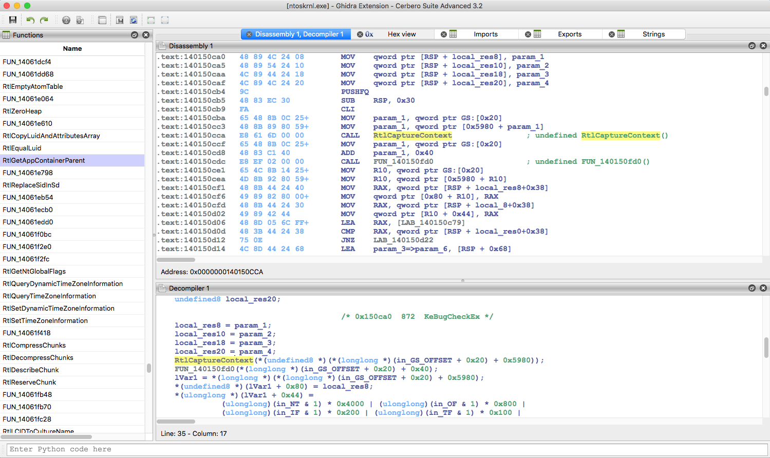
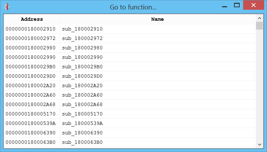
Ctrl+2 shows the list of functions:
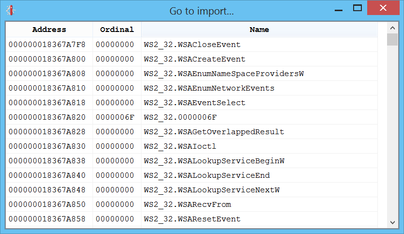
Ctrl+3 shows the list of imports:
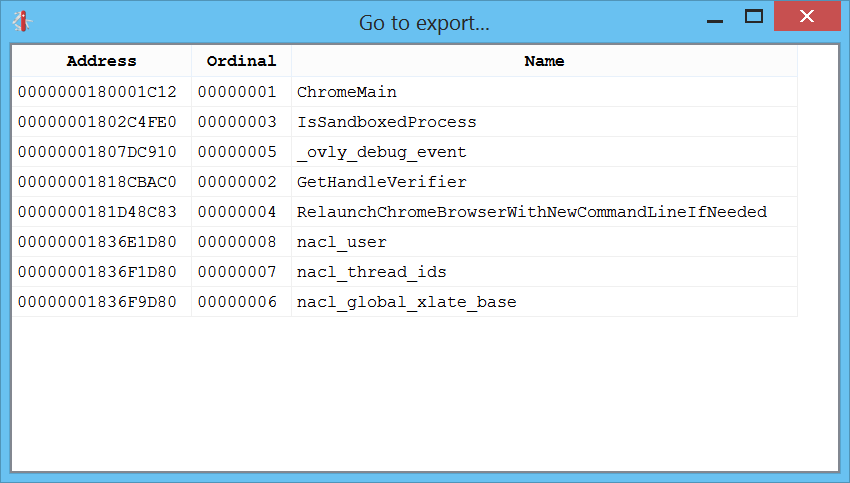
Ctrl+4 shows the list of exports:
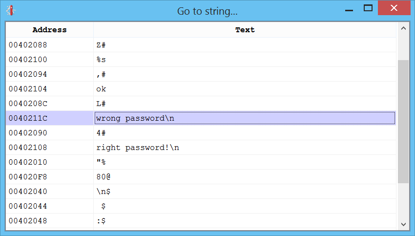
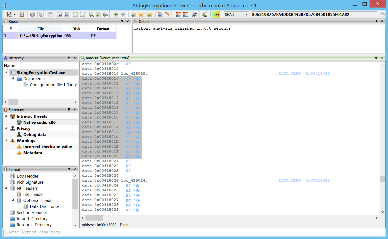
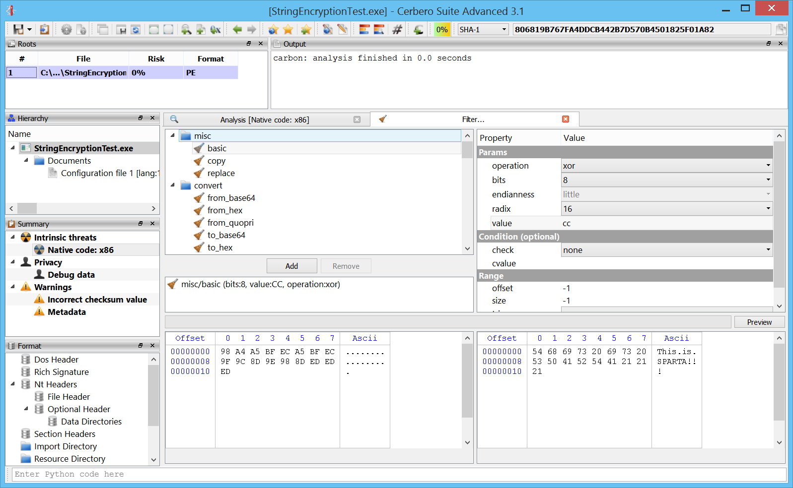
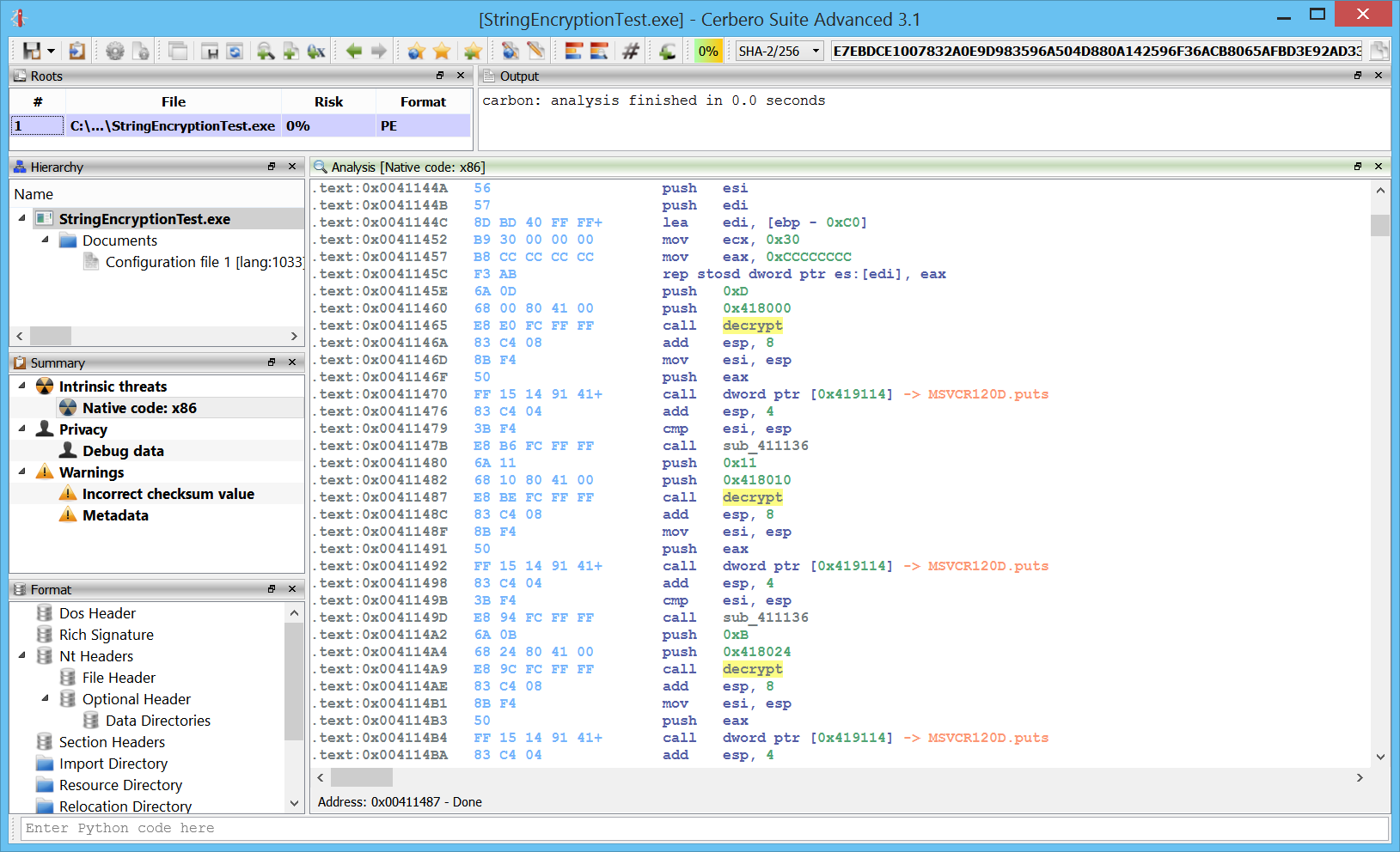
Strings
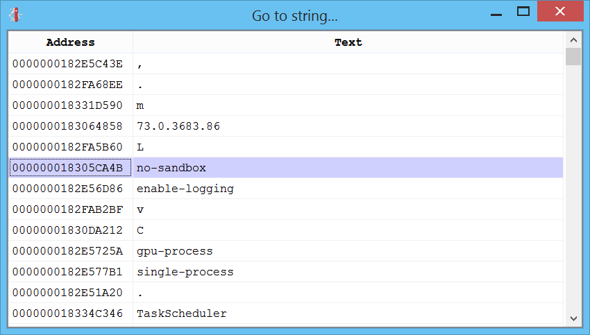
What about a good-old-days list of strings? That can be created by pressing “Ctrl+5”:
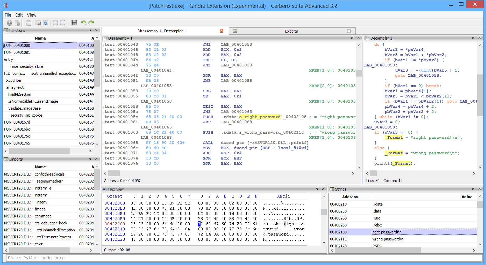
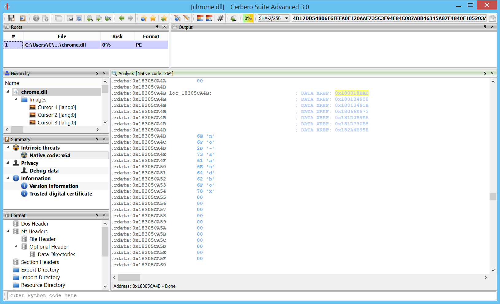
Once we jump to a string we can examine the locations in the code where it is used:
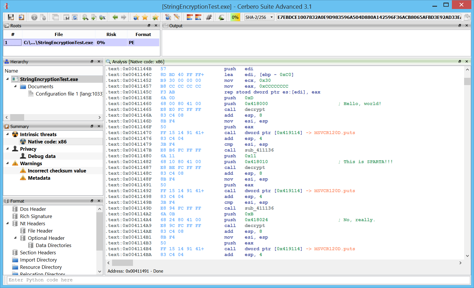
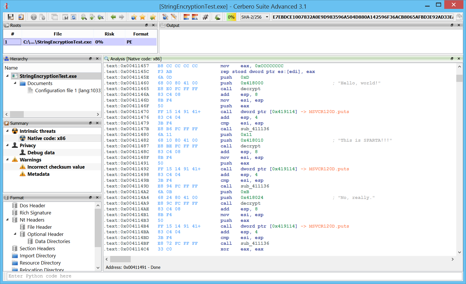
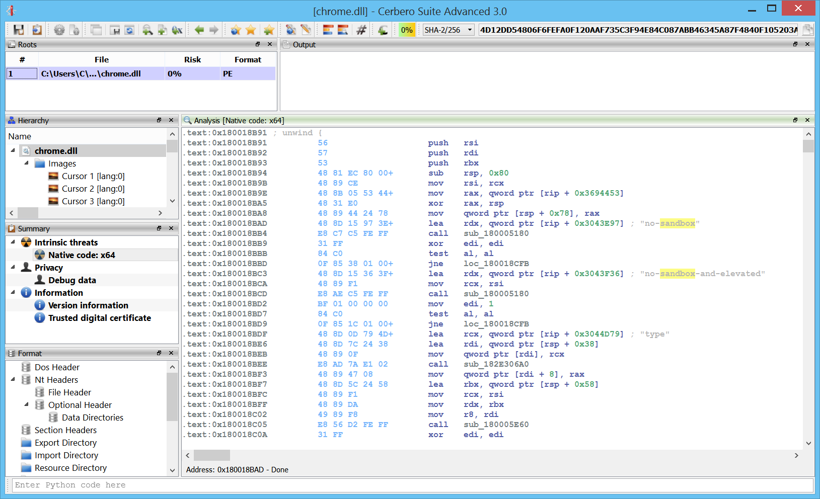
The disassembly itself will try to recognize strings and present them as self-generated comments whenever appropriate:
Integration
Great care has been taken to fit Carbon nicely in the entire logic of Cerbero Suite. Carbon databases are saved inside Cerbero Suite projects just as any other part of the analysis of a file.
While Carbon already provides support for flagged locations, nothing prevents you to use bookmarks as well to mark locations and jump back to them. The difference is that flagged locations are specific to an individual Carbon database, while bookmarks can span across databases and different files.
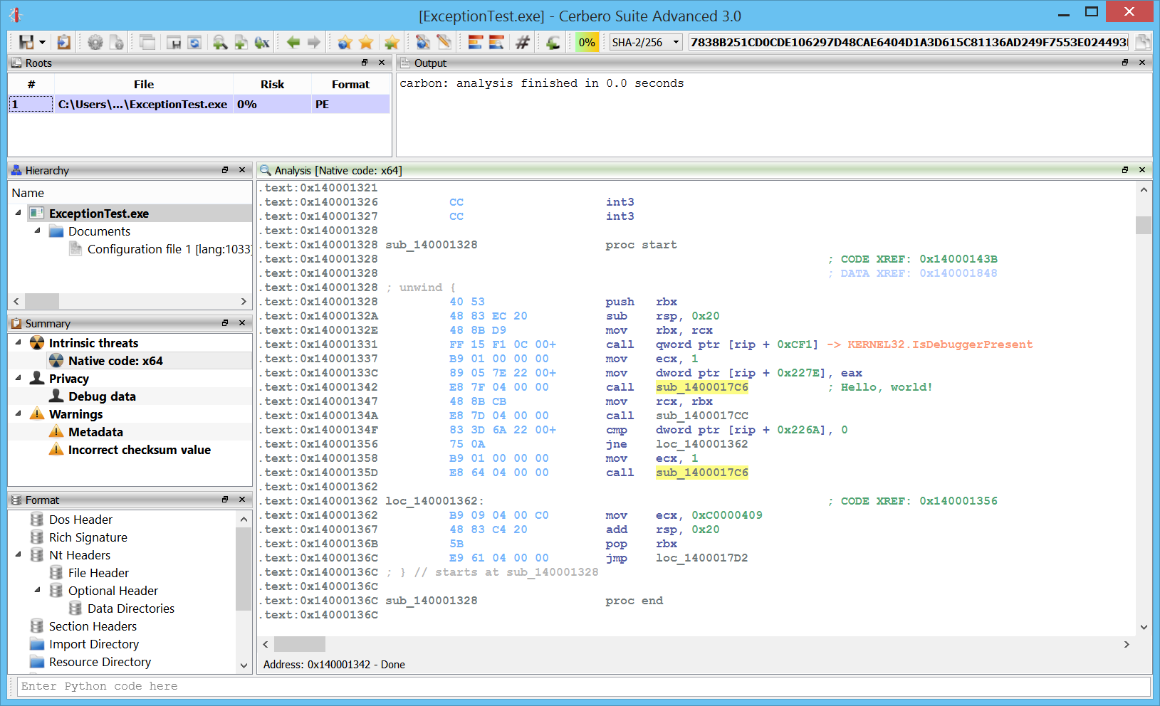
Themes
Last but not least: some eye candy. From the settings it’s possible to switch on the fly the color theme of the disassembly. The first release comes with the following four themes.
Light:
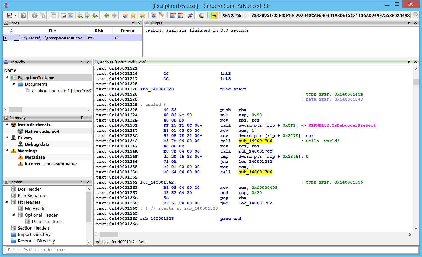
Classic:
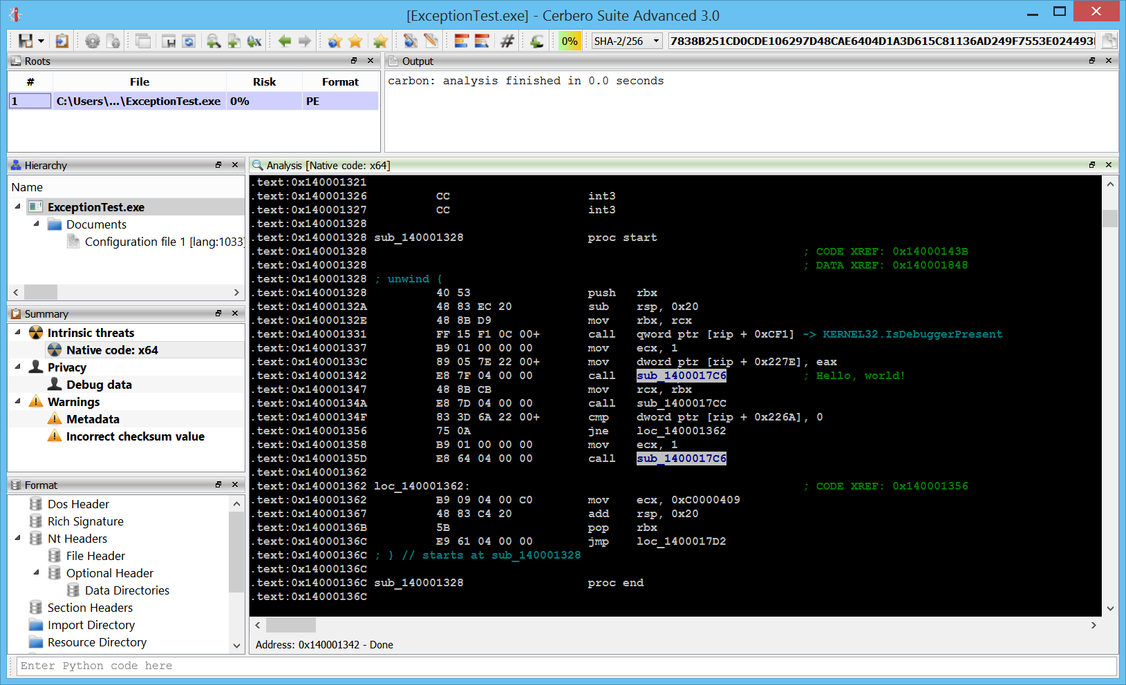
Iceberg:
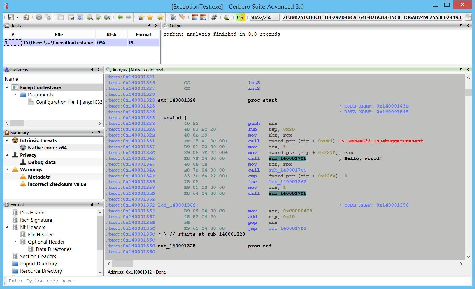
Dasm:
I’m sure that in the future we’ll be adding even more fun color themes. 🙂
Coming soon!